Word-to-Vector Embeddings II

Backpropagation

From the previous essay, we went through some layers, handling our data and using various weights and techniques to reach our initial guess at the true sentiment of a sentence (whether it is positive, negative or neutral). Next step, for any deep neural network, si simply to backpropagate, or see what changes we must make in our parameters in order to improve our guess. As always, we will use a Loss function, and an optimization algorithm in order to calculate the required gradients (if any of these terms are unclear, please go through my previous essays, or google for a brief understanding). We begin with defining our parameters and inputs, and working our way to a loss function. The transformation matrices below are simply a means to attaining the averaging and reduction.

\begin{array}{l} I n p u t V e c t o r : 𝐈 = {[\begin{array}{ccccc} i_{1} & i_{2} & i_{3} & \dots & i_{h} \end{array}]}_{1 * h} S p a r s e M a t r i x : {[\begin{array}{ccccc} 𝐒 \end{array}]}_{h * v} \\ T r a n s f o r m a t i o n M a t r i x_{1} : {[\begin{array}{c} 1 ⁄ x \\ 1 ⁄ x \\ 1 ⁄ x \\ ⋮ \\ 1 ⁄ x \end{array}]}_{x * 1} T r a n s f o r m a t i o n M a t r i x_{2} : [\begin{array}{c} 1 \end{array}] \\ W e i g h t s_{1} : {[\begin{array}{ccccc} w_{11} & w_{12} & w_{13} & \dots & w_{1 h} \\ w_{21} \\ w_{31} & ⋱ & ⋮ \\ ⋮ \\ w_{v 1} & \dots & w_{v h} \end{array}]}_{v * x} \end{array}

With the above given inputs and paramters, we can go through the forward propagation process again like so:

\begin{array}{l} E m b e d d i n g L a y e r : 𝐒 * 𝐖_{1} = 𝐇 \\ {[\begin{array}{ccccc} 𝐒 \end{array}]}_{h * v} {[\begin{array}{ccccc} w_{11} & w_{12} & w_{13} & \dots & w_{1 h} \\ w_{21} \\ w_{31} & ⋱ & ⋮ \\ ⋮ \\ w_{v 1} & \dots & w_{v h} \end{array}]}_{v * x} = {[\begin{array}{ccccc} 𝐇 \end{array}]}_{h * x} \\ G l o b a l A v e r a g e P o o l i n g : 𝐇 * 𝐓_{1} = 𝐆 \\ {[\begin{array}{ccccc} 𝐇 \end{array}]}_{h * x} {[\begin{array}{c} 1 ⁄ x \\ 1 ⁄ x \\ 1 ⁄ x \\ ⋮ \\ 1 ⁄ x \end{array}]}_{x * 1} = {[\begin{array}{c} g_{1} \\ g_{2} \\ g_{3} \\ ⋮ \\ g_{x} \end{array}]}_{x * 1} \\ R e d u c t i o n L a y e r : 𝐆 * 𝐓_{2} = 𝐎 \\ {[\begin{array}{c} g_{1} \\ g_{2} \\ g_{3} \\ ⋮ \\ g_{x} \end{array}]}_{x * 1} {[\begin{array}{c} 1 \end{array}]}_{1 * 1} = {[\begin{array}{c} o \end{array}]}_{1 * 1} \\ A c t i v a t i o n L a y e r : T a n h (𝐎) = 𝐏^{*} \\ \frac{e^{{[\begin{array}{c} o \end{array}]}_{1 * 1}} - e^{- {[\begin{array}{c} o \end{array}]}_{1 * 1}}}{e^{{[\begin{array}{c} o \end{array}]}_{1 * 1}} + e^{- {[\begin{array}{c} o \end{array}]}_{1 * 1}}} = [p^{*}] \end{array}

And with this, our model has given us it's very first guess of what the statement's sentiment can be. It's wrong, and we know it. We just need to let the model know how wrong it is, and in which direction it should go next in order to achieve better results. Our, or rather the model's next step will be calculating the gradients of the weights with respect to the lost function. We must therefore first define a loss function, and see how the actual gradient calculation would look like. For the loss function, we will use our dear old mean squared error, were we simply subtract our guess from the real value, where the real value is the true sentiment of the sentence. Let the true value be represented by **T**. With that, our loss function becomes,

L o s s : = {(𝐓 - \frac{e^{((𝐒 * 𝐖_{1}) * 𝐓_{1}) * 𝐓_{2})} - e^{- ((𝐒 * 𝐖_{1}) * 𝐓_{1}) * 𝐓_{2})}}{e^{((𝐒 * 𝐖_{1}) * 𝐓_{1}) * 𝐓_{2})} + e^{- ((𝐒 * 𝐖_{1}) * 𝐓_{1}) * 𝐓_{2})}})}^{2}

To begin with, we must recognize what our parameters are in the above equation, and what're the constants that are of no use to us. The paramter (in this case), is simply the weight matrix **W**₁, where as the other transformation matrices aren't really paramters but just helper matrices. **S** is our input, since it is constructed by taking in our sentence vector, and **T** is the ground truth, and hence the input and output are merely constants in the above equation (since we cannot change them in any way). With this, our next step becomes very simple: just calculate the gradient of the weight matrix with respect to the loss function:

\frac{δ L o s s}{δ 𝐖_{1}} = \frac{δ {(𝐓 - \frac{e^{((𝐒 * 𝐖_{1}) * 𝐓_{1}) * 𝐓_{2})} - e^{- ((𝐒 * 𝐖_{1}) * 𝐓_{1}) * 𝐓_{2})}}{e^{((𝐒 * 𝐖_{1}) * 𝐓_{1}) * 𝐓_{2})} + e^{- ((𝐒 * 𝐖_{1}) * 𝐓_{1}) * 𝐓_{2})}})}^{2}}{δ 𝐖_{1}}

This gradient is simple enough to calculate by hand, but thats not how our model will do it, so lets use our computer's method: making a computational graph, and using it to *back*-propagate in order to find our gradient. With defining the intermediate variables, we can make a computational graph for this particular model like this:

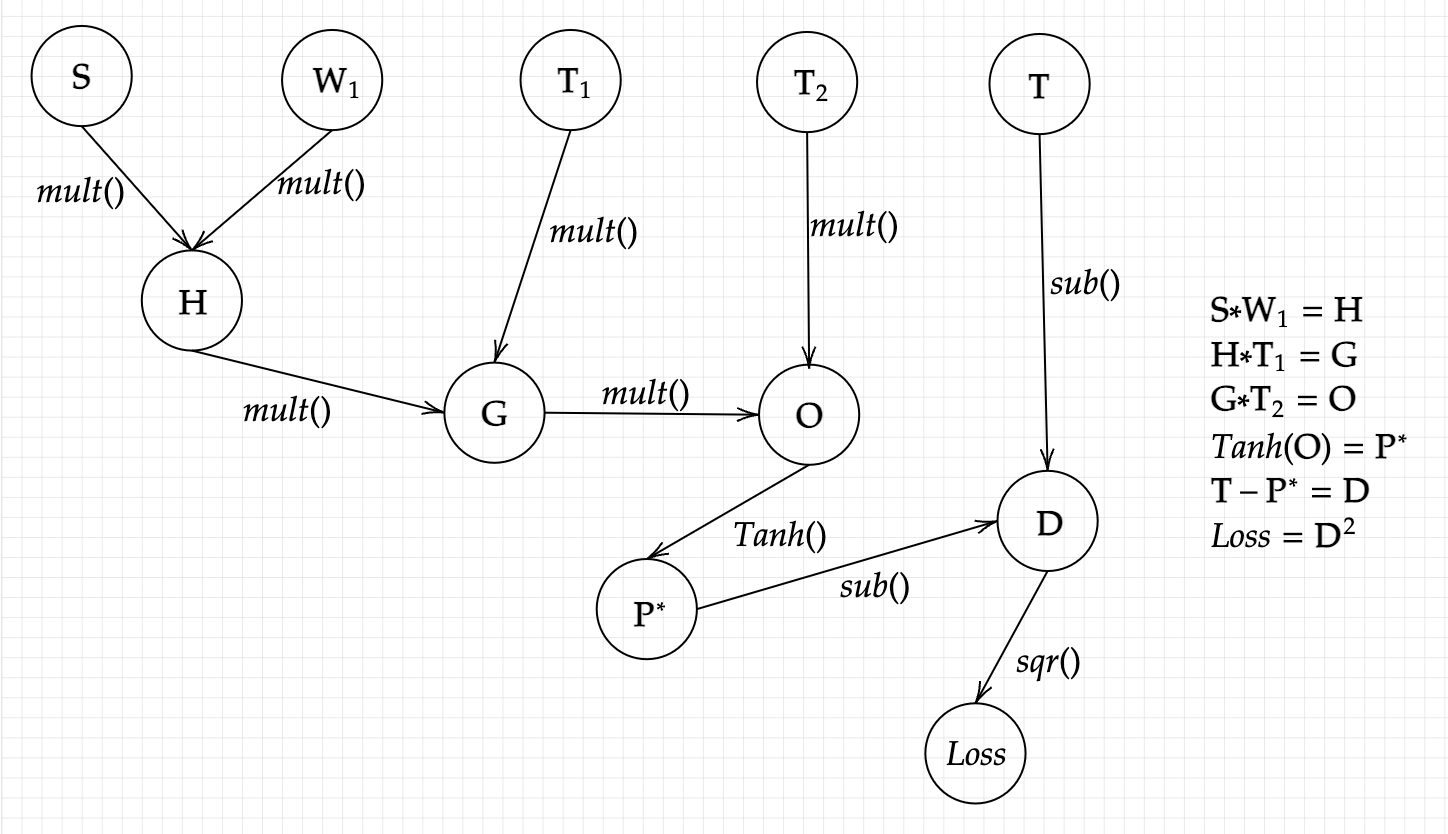And our desired gradient being :

\frac{δ L o s s}{δ 𝐖_{1}} = \frac{δ L o s s}{δ 𝐃} \frac{δ 𝐃}{δ 𝐏^{*}} \frac{δ 𝐏^{*}}{δ 𝐎} \frac{δ 𝐎}{δ 𝐆} \frac{δ 𝐆}{δ 𝐇} \frac{δ 𝐇}{δ 𝐖_{1}}

For the sake of simplicity, I have calculated the gradients for each inidivisual term,

\begin{array}{l} \frac{δ L o s s}{δ 𝐃} = \frac{δ 𝐃^{2}}{δ 𝐃} = 2 𝐃 \\ \frac{δ 𝐃}{δ 𝐏^{*}} = \frac{δ 𝐓 - 𝐏^{*}}{δ 𝐏^{*}} = 𝐓 - 1 \\ \frac{δ 𝐏^{*}}{δ 𝐎} = \frac{δ T a n h (𝐎)}{δ 𝐎} = 1 - T a n h^{2} (𝐎) \\ \frac{δ 𝐎}{δ 𝐆} = \frac{δ 𝐆 * 𝐓_{2}}{δ 𝐆} = 𝐓_{2} \\ \frac{δ 𝐆}{δ 𝐇} = \frac{δ 𝐇 * 𝐓_{1}}{δ 𝐇} = 𝐓_{2} \\ \frac{δ 𝐇}{δ 𝐖_{1}} = \frac{δ 𝐒 * 𝐖_{1}}{δ 𝐖_{1}} = 𝐒 \end{array}

Note: If this seems unfamiliar, readthis essay
And put them together in our final gradient, the term that will be subtracted from the weight matrix:

\frac{𝛅 𝐋 𝐨 𝐬 𝐬}{𝛅 𝐖_{𝟏}} = {𝐒 𝐓}_{1} 𝐓_{2} (2 (𝐓 - T a n h ((𝐒 * 𝐖_{1}) * 𝐓_{1}) * 𝐓_{2})) (𝐓 - 1) (1 - T a n h^{2} ((𝐒 * 𝐖_{1}) * 𝐓_{1}) * 𝐓_{2}))

Expanded:

With this, we have finally arrived at the last and final step of this iteration: to simply subtract this gradient form the weight matrix and *learn* from our mistakes (or rather the model's mistakes),

𝐖_{1} - \frac{𝛅 𝐋 𝐨 𝐬 𝐬}{𝛅 𝐖_{𝟏}}

Our model has finally learned from it’s mistake, ounce. We simply have to keep doing the results until we can get to sufficiently low loss function (but not zero, or too low).

Internal Meaning

After coming this far, you must be wondering, what on earth has this got to do with understanding language at all ? All we did was a bunch of linear algebra! Where was the part where our model/network understands language? You feel that way partly because we tackled this problem with pure mathematics, and hence it is very tough to see any intuitive meaning beyond what we see mathematically. If we had actually coded this model, it would still be a bit unclear. Thus for further clarity and to actually show what exactly did our model learn, and why this technique, though seemingly random at first, has very fascinating results, we can easily get an example. For this purpose, I had trained a model on the previous techniques (though I used some more layers), on a bunch of positive, negative and neutral sentences and had it guess the sentence’s sentiment. Our model, in order to guess the sentiment of a sentence, must find correlations between the words that make up the sentence, and use those correlations to predict the sentiment. For instance, it might associate the word ‘beautiful’ with a positive sentiment, and the word ‘terrible’ with a more negative sentiment, as in if these words appear in a sentence, the guess would slightly (or significantly, depends on the sentence), tilt towards the associated sentiment, i.e, a sentence with ‘beautiful’ in it might more probably be a positive one, and a sentence with ‘terrible’ in it will more probably be a negative one. So, we simply write a function that finds words that the model thinks are similiar to the word ‘beautiful’. Here are the results:

$\begin{array}{l} [(^{'} {𝐛 𝐞 𝐚 𝐮 𝐭 𝐢 𝐟 𝐮 𝐥}^{'}, - 0.0), (^{'} {𝐡 𝐨 𝐩 𝐞 𝐟 𝐮 𝐥 𝐥 𝐲}^{'}, - 0.5801912169518818), \\ (^{'} {𝐭 𝐡 𝐚 𝐧 𝐤}^{'}, - 0.6531024883061008), (^{'} {𝐰 𝐨 𝐧 𝐝 𝐞 𝐫 𝐟 𝐮 𝐥}^{'}, - 0.7246532646656508), \\ (^{'} {𝐜 𝐮 𝐭 𝐞}^{'}, - 0.8008494113576279), (^{'} {𝐠 𝐥 𝐚 𝐝}^{'}, - 0.8301763485770911), \\ (^{'} {𝐭 𝐡 𝐚 𝐧 𝐤 𝐬}^{'}, - 0.8305783412623376), (^{'} {𝐚 𝐰 𝐞 𝐬 𝐨 𝐦 𝐞}^{'}, - 0.8487631248615383), \\ (^{'} {𝐥 𝐨 𝐯 𝐞 𝐥 𝐲}^{'}, - 0.8681399020748348), (^{'} {𝐞 𝐧 𝐣 𝐨 𝐲 𝐢 𝐧 𝐠}^{'}, - 0.8888833737852143)] \end{array}$

And here are the results for using the same function on the word ‘terrible’:

$\begin{array}{l} [(^{'} {𝐭 𝐞 𝐫 𝐫 𝐢 𝐛 𝐥 𝐞}^{'}, - 0.0), (^{'} {𝐟 𝐚 𝐢 𝐥 𝐞 𝐝}^{'}, - 0.48034567707256337), \\ (^{'} {𝐲 𝐮 𝐜 𝐤 𝐲}^{'}, - 0.48587916470484127), (^{'} {𝐡 𝐮 𝐫 𝐭 𝐢 𝐧 𝐠}^{'}, - 0.4926016880220401), \\ (^{'} {𝐝 𝐞 𝐩 𝐫 𝐞 𝐬 𝐬 𝐢 𝐧 𝐠}^{'}, - 0.495007777206264), (^{'} {𝐥 𝐞 𝐚 𝐝 𝐞 𝐫 𝐬 𝐡 𝐢 𝐩}^{'}, - 0.5112371917188722), \\ (^{'} {𝐩 𝐨 𝐨 𝐫 𝐥 𝐲}^{'}, - 0.5235972401092943), (^{'} {𝐝 𝐞 𝐩 𝐫 𝐞 𝐬 𝐬 𝐞 𝐝}^{'}, - 0.5243161177963896), \\ (^{'} {𝐭 𝐚 𝐤 𝐞 𝐫 𝐬}^{'}, - 0.5266746153705941), (^{'} {𝐫 𝐮 𝐢 𝐧 𝐞 𝐝}^{'}, - 0.5276953714430769)] \end{array}$

The first time I saw this results, I was amazed! It was just mind-blowing how, after doing seemingly very simple math(!), like linear algebra, a computer program was able to find (or guess?) the intrinsic meaning of words! From the above results, we can clearly see that our model has correctly (somewhat) found correlations between certain words, and how these words have certain underlying meanings that could be captured in a weight matrix. The model was able to determine that the words ‘beautiful’, ‘wonderful’ and ‘lovely’ have a certain correlation with being positive, and certain other words like ‘terrible’, ‘depressed’ or ‘ruined’ are more similiar, as they are correlated with being negative. If you notice, it also associated the word ‘leadership’ with ‘terrible’, that could be mistake, OR that word was more likely used in a negative statemant. Mind you, this is a very rudimentary model, trained for only 10 iterations, and still produced such wonderful results! As we add more layers (make it more complicated), or use different architectures, we can be ever so close to understanding some portion of our natural language.

Home