Exploring architectures- Transformers II

Queries, Keys and Values

The most important concept that the attention mechanism introduces is familiar with the computer science community since ages: that of queries, keys and values. Note: whenever I say token, I am referring to either a word or a letter, something that needs to be predicted/generated. Each token has it’s own query, keys and values, which are used to calculate it’s self-attention weights, essentially a matrix/vector that captures it’s relation with every other token. These are than used to either decode (in case of translation) or generate other tokens. Before going through the calculation of these weights, let us declare important weight matrices. These are used to calculate the Query, Key and Value for each token. The same weight matrices are used on every token.

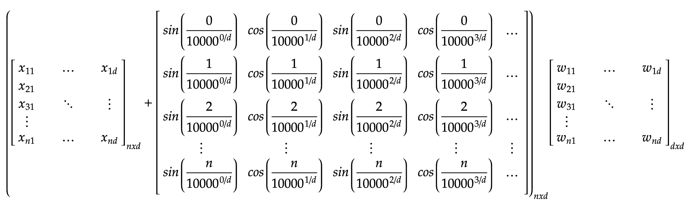
{𝐖_{𝐕} = 𝐖_{𝐊} = 𝐖}_{𝐐} = {[\begin{array}{ccccc} w_{11} & \dots & w_{1 d} \\ w_{21} \\ w_{31} & ⋱ & ⋮ \\ ⋮ \\ w_{d 1} & \dots & w_{d d} \end{array}]}_{d x d}

The forward propagation is fairly easy: each token’s query is used to get the dot product similiarity between that query and the keys of all other tokens, and the resultant vector will be used with the value matrix of that token to get the self-attention weights of the token. this would conclude the weight calculation. In order to further predict or generate, we simply pass the desired weights through a dense network to get our output. The details of these operations would be discussed below. Let us begin with calculating the Query, Key and Value matrix for each token, by matrix multiplication with the addition of our input matrix and the positional matrix, X+P. Remember, X has n tokens, each of which is represented by a d-dimensional vector. Hence it’s dimensions are (n x d).

\begin{array}{l} 𝐐 = ({𝐗 + 𝐏) 𝐖}_{𝐐} \\ 𝐊 = ({𝐗 + 𝐏) 𝐖}_{𝐊} \\ 𝐕 = ({𝐗 + 𝐏) 𝐖}_{𝐕} \end{array}

The next step would be to get the dot product attention between the Query matrix and the Key matrix. Here we perform a batch matrix multiplication between the Query and the Key matrix to get the similiarity values of every token with every other token, essentially giving us an n x n matrix.

{𝐐 𝐊}^{𝐓} = {[\begin{array}{ccccc} q_{11} & \dots & q_{1 d} \\ q_{21} \\ q_{31} & ⋱ & ⋮ \\ ⋮ \\ q_{n 1} & \dots & q_{n d} \end{array}]}_{n x d} {[\begin{array}{ccccc} k_{11} & \dots & k_{1 n} \\ k_{21} \\ k_{31} & ⋱ & ⋮ \\ ⋮ \\ k_{d 1} & \dots & k_{d n} \end{array}]}_{d x n}

Before we multiply with the value matrix, we scale this matrix with 1/srqt(d), to bring the overall variance to one and apply the softmax operation in order to limit the values within a probability distribution. Further, we simply multiply the resultant matrix with the Value matrix. This gives us the self-attention weight matrix, which captures the relationship between all the tokens, be it letters or be it words. (ϕ denotes the softmax function).

ϕ (\frac{{𝐐 𝐊}^{𝐓}}{\sqrt{d}}) 𝐕

Going forward, we also add back the input, essentially as a residual connection.

ϕ (\frac{{𝐐 𝐊}^{𝐓}}{\sqrt{d}}) 𝐕 + 𝐗

This is to be followed by layer normalisation. In the transformer, the process of addition of residual connection and the layer normalisation happnens in the same layer, known as an AddNorm layer. (The normalisation happens layer-wise, that is, row wise).

\frac{(ϕ (\frac{{𝐐 𝐊}^{𝐓}}{\sqrt{d}}) 𝐕 + 𝐗) - μ}{σ}

At this stage, it would help for us to visualise the above given equation purely in terms of the weight paramters and the input:

\frac{(ϕ (\frac{((𝐗 + 𝐏) 𝐖_{𝐐}) (({𝐗 + 𝐏) 𝐖}_{𝐊})^{𝐓}}{\sqrt{d}}) (({𝐗 + 𝐏) 𝐖}_{𝐕}) + 𝐗) - μ}{σ}

NOTE: If terms like layer normalisation, residual connection or positional encoding seem unfamiliar, read the previous essay.

Getting the output

At the end of the last step, the addnorm layer, we do not yet have our final output. Remember: we need a d-dimensional vector, which represents a token to be generated or predicted at the end, and we have a n x d dimensional matrix. Thus we need to pass this matrix through a dense neural network in order to get to our final output, which just means multiplying the matrix with another weight matrix. The weight matrix could be of dimensions *(d * v)*, where v is the vocabalry size. (Vocabulary size just refers to the size of a dictionary object, which indexes the entire corpus of tokens used). Thus we are left with :

𝐖 = {[\begin{array}{ccccc} w_{11} & \dots & w_{1 v} \\ w_{21} \\ w_{31} & ⋱ & ⋮ \\ ⋮ \\ w_{d 1} & \dots & w_{d v} \end{array}]}_{d x v}

(\frac{(ϕ (\frac{((𝐗 + 𝐏) 𝐖_{𝐐}) (({𝐗 + 𝐏) 𝐖}_{𝐊})^{𝐓}}{\sqrt{d}}) (({𝐗 + 𝐏) 𝐖}_{𝐕}) + 𝐗) - μ}{σ}) 𝐖 = {[\begin{array}{ccccc} o_{11} & \dots & o_{1 v} \\ o_{21} \\ o_{31} & ⋱ & ⋮ \\ ⋮ \\ o_{n 1} & \dots & o_{n v} \end{array}]}_{n x v}

The output matrix (let’s call it O) is of the dimensions n x v because: there are n tokens and the size of the vocabalury object is v. The output has the prediction of the token that comes after the nth token, for example, the first token in O is the one that the model predicted should come after the first token in X, and so on. The generated token at the last, or the nth token in O is the one that comes after the nth token in X, and hence the true predicted token. The previous tokens are predicted in order to compare it with the actual tokens, and learn from the errors. These predicted tokens are now to be compared with the actual tokens. During the training process (as you may have guessed), we stop one token before the last, in order to learn the gradients, as the last token would be the true value that the nth token in O will be compared with.

Loss function

Since the cross entropy loss is taken to be between the predicted probability distribution and the true probability distribution, we must pass our matrix through a softmax function, but applied across each rows, in order to constrain them in a distribution, which is to be compared with T, the true probability distribution. (It’s rows have the one-hot encodings of the actual tokens used).

𝐎 = {[\begin{array}{c} ϕ ([\begin{array}{ccccc} o_{11} & o_{12} & o_{13} & \dots & o_{1 v} \end{array}]) \\ ϕ ([\begin{array}{ccccc} o_{21} & o_{22} & o_{23} & \dots & o_{2 v} \end{array}]) \\ ϕ ([\begin{array}{ccccc} o_{31} & o_{32} & o_{33} & \dots & o_{3 v} \end{array}]) \\ ⋮ \\ ϕ ([\begin{array}{ccccc} o_{n 1} & o_{n 2} & o_{n 3} & \dots & o_{n v} \end{array}]) \end{array}]}_{n x v} 𝐓 = {[\begin{array}{ccccc} t_{11} & \dots & t_{1 v} \\ t_{21} \\ t_{31} & ⋱ & ⋮ \\ ⋮ \\ t_{n 1} & \dots & t_{n v} \end{array}]}_{n x v}

We take the cross-entropy loss between each row (this these are the distributions) and than simply take the means of the resultant loss vector to finally get to the Loss, which can be backpropgated with.

𝐋 = - {[\begin{array}{c} (𝐭_{1} \times l o g (𝐨_{1})) {[\begin{array}{c} 1 \\ ⋮ \\ 1 \end{array}]}_{v x 1} \\ (𝐭_{2} \times l o g (𝐨_{2})) {[\begin{array}{c} 1 \\ ⋮ \\ 1 \end{array}]}_{v x 1} \\ (𝐭_{3} \times l o g (𝐨_{3})) {[\begin{array}{c} 1 \\ ⋮ \\ 1 \end{array}]}_{v x 1} \\ ⋮ \\ (𝐭_{n} \times l o g (𝐨_{n})) {[\begin{array}{c} 1 \\ ⋮ \\ 1 \end{array}]}_{v x 1} \end{array}]}_{n x 1}

Summing across the column, and dividing by it’s length, we get the final loss value.

L o s s = \frac{1}{n} \sum_{i = 1}^{n} 𝐋_{i}

Backpropagation

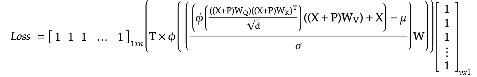
As is the case, we shall now backpropagate through the loss function in order to calculate the gradients of each weight parameter, with respect to the loss function. Before moving on, let us ounce again look at our final loss function, in terms of only the input, true values and the weights. In case you’re wondering, the first and the last vector of ones simply help in the addition of the row and column values, and reduce the matrix into a single scalar value: our loss.

We proceed with constructing a computational graph in order to find the gradients of these weights: WQ, WK, WV and W, which are:

\frac{δ L o s s}{δ 𝐖_{𝐐}} \frac{δ L o s s}{δ 𝐖_{𝐊}} \frac{δ L o s s}{δ 𝐖_{𝐕}} \frac{δ L o s s}{δ 𝐖}

The graph given below traces the intermediate variables (as they would’ve formed in the autograd process), and makes it much easier to calculate the gradients.

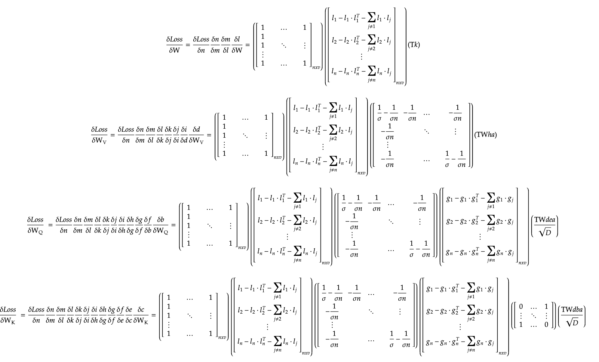
Following this backpropagation process, we trace the edges (lines) backwards to each node, and collect the subsequent gradients till we reach the desired nodes of the weights. Few points to consider in the below given equations: the matrix dimensions may not seem to align, but that’s simply bacause I’ve calculated the gradients as is, we are free to perform any transpositions (to eventually match the dimensions of the parameters). The letters given below are simply the intermediate variables defined in the above image, I have not substituted them back to save space. With that said, here are the gradients of the four parameters:

Conclusion

This is the last major architecture that is widely used in the industry. Transformers was truly a revolution in the machine/deep learning community and to our entire world: we saw a glimpse of true artificial intelligence. Although this may seem hopeful, we are still far from acheiving the goal of artificial intelligence. To someone who has read these essays simply, without any exposure to outside community, it might seem that transformers are just another form of algorithmic equations that solve some problems faced in previous one: but practical application makes all the difference. There are many more models and techniques to explore (even though they may not widely be known) and I will continue this journey to find and write about new architectures and techniques in this field. Thank you.

Home