Exploring architectures- Transformers

Introduction

“Necessity is the mother of all invention.”
As we discussed in the last essay, LSTMs were the go to model architectures that were used in sequential tasks such as natural language processing and time-series data. But as we scaled the tasks and datasets, LSTMs struggled to keep up. The main problem turned out to be context-length, it proved difficult for LSTMs to ‘remember’ long contexts, and thus anything learned in the earlier data points was forgotten or simply lost during the forward propagation and the subsequent backpropagation method. This problem, we can also call this the vanishing gradient problem, could also be mitigated with the use of a residual network (explained further in the essay) on a LSTM network, but this did little to help retain the information from earlier layers and hence it continued to suffer from this issue. First proposed by Bahadanau et al in 2014, a new solution popped up: the attention mechanism, and it led to a new area of research for the course of the following years until 2017, when Vaswani et al proposed a new architecture, leading to a near exponential growth in the AI community. In this essay we explore, mathematically as usual, this new architecture and it’s related techniques. Since there is a lot to explore, this essay will be long, so be prepared! That said, we will gain a thorough understanding of the infamous Transformer architecture in return.

A problem and a solution

As discussed before, we had a problem at hand. The previous architectures failed to capture and retain the information learned in the earlier stages of training, as the input/context got longer and as we trained on more and more data. This was especially problematic with natural language, as we cannot afford to loose any information at all: even a word missing from a sentence completely changes the meaning, for example: “Don’t eat that” just becomes “eat that”. In longer contexts, words/input/token or simply information, if forgotten, can simply yield inaccurate or wrong results. LSTMs suffered from this issue and hence performed poorly on certain tasks. A proposed solution was using the attention mechanism, whose primary principle is to form connections between a word and every other word in a sentence, in essence, capture the relationship between all the words in a parameter. In this sense, all the words would have connections with all the other words, captured in what we call a self-attention weights of that word/input/token. This eliminates the problem of vanishing gradients, as the information cannot be forgotten, since unlike in LSTMs, these connections (for the calculation of self-attention weights) are directly established (as opposed to indirect establishment throught intermediate parameters). This has another benefit: the entire process of calcualting these self-attention weights for each word (with every other word) can be done in parallel, for example, if we are calculating these weights for the first word, nothing stops us from doing the same for the second and third words as well, since these calculations are independant of each other. This helps us distribute these operations into specialized hardwares (GPUs) and hence speed up training.

Encodings and Embeddings

The main aim for this architecture was initially to tackle natural language tasks, which meant dealing with words. As discussed in many previous essays, the words are represented by d-dimensional vectors, also known as word embeddings. These embeddings help us transition from the world of letters and alphabets to a world of vectors, where our models can work their magic. These word embeddings are to be the input to our model. Before the propagation begins, we must ensure one more thing. Transformers do improve on LSTMs and RNNs, but unlike these models, they fail to preserve the order of the words or letters in a given input. As mentioned before, self-attention weights are calculated for each token (could be a word or a letter) with respect to every other token, hence the order is not preserved, i.e, the model does not take into account which word comes after another. We did not face this issue in LSTMs as the hidden state was passed only in one way: forward, from one token to another, but in the Transformer architecture, parallel computing is favoured, hence every self-attention weight is calculated simultaneously, and therefore we must somehow encode the positional information of a word into the model. This step is known as Positional Encoding. In order to encode the position of a token within a sentence or a word, we use sin and cos functions. With the intention being clear, the actual operation is pretty simple. Let us first define an input matrix X, of dimensions (n x d). This simple means there are n tokens, each of which is represented by d dimensional vector. The token could be a word or just a letter. The vector representation could come from a variety of techniques (one could be this). With this matrix done, we must create our positional matrix. This matrix, P would be of the same dimensions as our input matrix (n x d). We initialise this matrix in the form of zeroes. Following that, we simply perform a certain sin() and cos() functions like so:

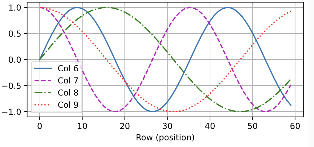
𝐏 = {[\begin{array}{ccccc} 0 & \dots & 0 \\ 0 \\ 0 & ⋱ & ⋮ \\ ⋮ \\ 0 & \dots & 0 \end{array}]}_{n x d}

Now on every odd column, we perform a sin() function, and on every even column, we perform a cos() function. In order to understand what’s happening, recall that sin and cos are waves on a graph. Waves with low and high frequency. What we do here, is simple add a higher frequency wave to our first token, and keep lowering the frequency as we go forward to each token. This essentially gives each token a unique and specific order (the order of the sin and cos waves) and in a way encodes their position. The functions are given below.

𝐏 = {[\begin{array}{ccccc} s i n (\frac{0}{10000^{0 / d}}) & c o s (\frac{0}{10000^{1 / d}}) & s i n (\frac{0}{10000^{2 / d}}) & c o s (\frac{0}{10000^{3 / d}}) & \dots \\ s i n (\frac{1}{10000^{0 / d}}) & c o s (\frac{1}{10000^{1 / d}}) & s i n (\frac{1}{10000^{2 / d}}) & c o s (\frac{1}{10000^{3 / d}}) & \dots \\ s i n (\frac{2}{10000^{0 / d}}) & c o s (\frac{2}{10000^{1 / d}}) & s i n (\frac{2}{10000^{2 / d}}) & c o s (\frac{2}{10000^{3 / d}}) & \dots \\ ⋮ & ⋮ & ⋮ & ⋮ & ⋮ \\ s i n (\frac{n}{10000^{0 / d}}) & c o s (\frac{n}{10000^{1 / d}}) & s i n (\frac{n}{10000^{2 / d}}) & c o s (\frac{n}{10000^{3 / d}}) & \dots \end{array}]}_{n x d}

If we were to graph the waves, they’ll look like the image given below. Note that each line is of a different frequency, and that higher columns have lower frequency (they are alternating sin and cos waves, with lowering frequency).

The first step of our architecture is therefore simply :

𝐗 + 𝐏

Residual Connections

Vanishing gradients has been a problem since before transformers. Gradients, on wider and deeper networks have a high chance of disappearing or vanishing, that is, they go to zero. This leads to information loss, and hence undesirable. One genuis solution, and simple, was to simple add back the input (the very first, initial input) back to the output at the very end of the network. An example: suppose we have a network that takes our input X to an output: *g(X)*. Now, we add X back into *g(X)*, to give us *f(X)*.

f (𝐗) = g (𝐗) + 𝐗

The intuition behind doing so is this: our task is to guess our input X, and *g(X)* is supposed to be our matrix equation, upon solving which, we get our best guess. Suppose we say that our intial network is simply an equation like Ax = b. This means our goal is to make b as close to x as possible, through the transformation matrix A. Normally, thus we perform a search in the column space of the weights matrix in order to find the solution, namely the weights of the matrix A. So, we add in x again, at the end like so:

𝐀 𝐱 + 𝐱 = 𝐛

Now, in order to guess our weights for the matrix A, we subtract the equation by x.

𝐀 𝐱 = 𝐛 - 𝐱

Now taking into consideration that our goal is to take our output as close to x as possible, our goal becomes:

𝐛 = 𝐗 o r f (𝐗) = 𝐗

Which is essentially the identity mapping, and is far simpler to calculate. Notice, that this also means that

g (𝐗) = 0 o r 𝐀 𝐱 = 𝟎

And we search in the null space of our residual connection. This might have certain advantages, such as solving a homogenous set of equations and might be less computationaly expensive, but our main goal was to introduce the identity mapping and take care of the vanishing gradient problem. There is no loss of information in this regard, as the input is added after all the operations have taken place.

Note: the network does NOT explicitly search in the Null space, but it CAN be intepreted that way in some cases. The main focus is learning the more easier identity mapping and solving the vanishing gradient problem

Layer Normalization

Another extremely useful technique was to apply layer-wise normalisation. This is a simple process (also used in the original paper Attention is all you need). Suppose we have a d-dimensional vector. This technique simply standardises the numbers within the vector by applying the well-known formula :

\frac{𝐱 - μ}{σ}

This is applied to the entire vector. The mean and variance are calculated by the below given formula :

\begin{array}{l} μ = \frac{1}{d} \sum_{i = 1}^{d} x_{i}, σ = \frac{1}{d} \sum_{i = 1}^{d} (x_{i} - μ)^{2} + ϵ \\ w h e r e \\ ϵ > 0 \end{array}

Layer normalisation has several benefits, like keeping the gradients in check, while also easing the flow of gradients within the network. It also helps in convergence of the weight paramters to their optimal value, where the loss is at ta desirable level.

Similiarity Functions

One of the steps going forward will be getting a numeric quantity for measuring the similiarity between two vectors. The vectors in this case may represent a word or a sentence, where we might want to measure the similiarity of the vector representations of those letters or words. The method is to simply take the dot product of the matrices. The intuition is pretty simple: the vectors which face in the same direction (that is, are similiar), give positive values, the vectors that are in the opposite direction give negative values, and the vectors that are perpendicular to each other given zero: they are not similiar at all. Finally, we assume that the vectors are independantly drawn identical variables, with zero mean and a variance of 1 x the number of dimensions. Thus to normalise the vector, we simply divide by the square root of the number of dimensions.

{[\begin{array}{c} a_{1} \\ a_{2} \\ a_{3} \\ ⋮ \\ a_{d} \end{array}]}_{d x 1} \times {[\begin{array}{c} b_{1} \\ b_{2} \\ b_{3} \\ ⋮ \\ b_{d} \end{array}]}_{d x 1} = \frac{\sum_{i = 1}^{d} a_{i} b_{i}}{\sqrt{d}}

With that, we are done with most of the helper functions that will be used in the architecture. The forward propagation step, it’s intuition and mathematical perspective will be explored in the next essay.

Continure Reading
Home