Neural Networks with Linear Algebra

The following essay will be an attempt in looking at Neural Networks through the lens of Linear Algebra. Neural Networks (or Machine Learning in general) are mathematically defined and can also be seen as an application of Linear Algeba itself, with the amalgation of calculus resulting in Vector Calculus. Learning this topic through a mathematical viewpoint often leads to understanding of the why of Neural Networks (or Machine Learning in general), why certain formulas are applied/used, and why they are effective. The knowledge behind how is mostly grounded in computer science, and fascinating though it is, I will mostly try to avoid it. The programming, data structures and algorithms utilized for implementing the concepts in Linear Algebra will not be covered in this essay.

Part I

Neural Networks, in the most rudimentary sense, take in an input, and return an output. The output is generally termed as a prediction. The output can be the same variable as an input, as in predicting tomorrow’s stock price, or it can be something different, i.e, if a given image is a cat or a dog (the input being image). What does a Neural Network do ? For now, it takes in a number, multiples it with another number, and gives an output.

$$[x][w]=[o]$$

Above, X is the input, W is the number to be multiplied, termed as a weight, and O is the output. This is the beginning of any Neural Network, take the input and multiply it by the weight. The output is the prediction. We have predicted something (however wrong it may be) and must therefore somehow check how wrong or far from the true value we are. This can be achieved by comparing our prediction with the true value. It is the actual value of the thing we are trying to predict. For example, we predicted a dog, but what actually was the image? Or what was today’s actual stock price ? We compare our output, with the actual value of the variable. How ? Well there are many ways. In fact, how we calculate the error is extremely crucial, so much so that it can actually help you nudge the Neural Network in the direction you want it to learn ! In this case, we simply take the difference,

$$[true-o]$$

Both variables being numbers, the result can take any real integer value. The error has another term: Loss function. But there is a problem, that the error can take negative values. We only want the distance (how much) between the prediction and the true value, not the direction (yet). Therefore, we simply square the value,

$$Loss=[true-o{]}^2$$

This is the complete loss function. Math is simple isn’t it ? Now let’s continue further. You may be wondering, what is so “Linear Algebra” about this? Well here it is. I have restricted the size of the input (or the output), but the input can also be a Vector.

$$X={\left[\begin{array}{ccccc}{x}_1& x_2& x_3& \dots & x_n\end{array}\right]}_{1*n}^T$$

The T indicates that it’s a column vector (not a rule, but is generally used) so it’s a notation for transpose. The output can also be a vector, though it depends on what we are trying to predict. In some cases, it’s a single variable and in others, it’s a vector. Now because of the laws of matrices, our prediction are,

$${\left[\begin{array}{c}{x}_1\\ x_2\\ x_3\\ ⋮\\ x_n\end{array}\right]}_{1*n}^T{\left[\begin{array}{ccccc}{w}_{11}& w_{12}& w_{13}& & w_{1z}\\ w_{21}& & & & \\ w_{31}& & \ddots & & ⋮\\ & & & & \\ w_{n1}& & \dots & & w_{11}\end{array}\right]}_{n*z}={\left[\begin{array}{c}{p}_1\\ p_2\\ p_3\\ ⋮\\ p_z\end{array}\right]}_{1*n}^T$$ $$n,z\in \mathbb{N}$$

The dimensions of the weight are easy to calculate, they are simply (number of elements of Input x number of elements of Output). Here, we are at the beginning of Linear Algebra. We normally also add in some weights, as it helps in getting more accurate results.

$${\left[\begin{array}{c}{x}_1\\ x_2\\ x_3\\ ⋮\\ x_n\end{array}\right]}_{1*n}^T{\left[\begin{array}{ccccc}{w}_{11}& w_{12}& w_{13}& & w_{1z}\\ w_{21}& & & & \\ w_{31}& & \ddots & & ⋮\\ & & & & \\ w_{n1}& & \dots & & w_{11}\end{array}\right]}_{n*z}+{\left[\begin{array}{c}{b}_1\\ b_2\\ b_3\\ ⋮\\ b_z\end{array}\right]}_{1*z}^T={\left[\begin{array}{c}{p}_1\\ p_2\\ p_3\\ ⋮\\ p_z\end{array}\right]}_{1*n}^T$$

The column vectors with b’s in it is called the bias or the bias vector. Since it is an addition, it has the same dimensions as the output, and lastly, our Loss function becomes,

$$({\left[\begin{array}{c}{t}_1\\ t_2\\ t_3\\ ⋮\\ t_{nz}\end{array}\right]}_{1*z}^T-{\left[\begin{array}{c}{e}_1\\ e_2\\ e_3\\ ⋮\\ e_z\end{array}\right]}_{1*z}^T)={\left[\begin{array}{c}{e}_1\\ e_2\\ e_3\\ ⋮\\ e_z\end{array}\right]}_{1*z}^T$$

But, this returns another vector. What we are looking for is a single number to measure the overall loss of the entire network, not just indivisual values. Thus we simply add all the elements in the resultant vector, and divide it by the number of elements, in other words, take the average.

$$Loss\text{}=\frac{{\sum }_{i=0}^z{e}_i}{z}$$

With this, we have a loss function with multi-dimensional outputs. This particular loss function is called the Mean Squared Error (MSE). The MSE is how bad our prediction is. The bigger the loss, worse is the prediction, and hence, we must somehow reduce or minimize the error. This brings us to perhaps the most crucial part of Machine Learning, or Artificial Intelligence in general, the Learning part. By somehow minimizing this error, the network learns from it’s mistakes, and makes better and better predictions. But how ? How do we reduce the error ? The answer is hidden in calculus.

Part II

What is a derivative ? It is the slope of a curved line. But another way of looking at it, is that a derivative is simply a way to establish a relationship between a function, and it’s variables. Let’s see a simple example,

$$y=w^{2}orf(x)=w{\text{}}^2$$

A function contains a variable, W. The variable changes. How much, and in which direction will the function change ? If we change W, how will the function f(W) or W² change ? If W is 4, the function is 16. If W is 6, the function is 36. Here, we have to encapture how much and in which direction does the function change. The answer is to find the derivative of the function with respect to W. The formulas and intuitions won’t be explained here, but the derivative is 2W in this case. It is denoted by d/dw.

$$\frac{d}{dx}f(x)=2w$$

A function with multiple inputs ? Same answer. Find the derivative with respect to the variable concerned.

$$z=w^2+y^2$$

For Y’s impact on Z, we find,

$$\frac{\delta }{\delta y}Z=2y$$

For W’s impact on Z, we find,

$$\frac{\delta }{\delta w}Z=2w$$

The method or steps to calculate derivatives, normal or partial (with multiple variables) are simple enough, so I won’t be going through them in this essay. The derivative of W and Y basically tells us that if we increase them by one unit, how much will it affect Z, will it increase ? or decrease ? and by how much ? From the example above, we see that if W increases, Z multiplies by 2 times W, same with Y. Imagine, that Z is the loss function, and W and Y are variables we can control. This means that if we tweak them properly, we can minimize the loss ! If we tweak the W and Y variables in a certain direction by a certain amount, the result will be a decrease in the loss function (which is Z in this case). The change/tweak in those variables will basically be a decrement by their derivatives.

$$\begin{array}{l}W-\frac{\delta }{\delta y}Z\\ Y-\frac{\delta }{\delta w}Z\end{array}$$

By doing the above mentioned operation, we have decreased the loss ! Or decreased the Z function. Now, let us compare this to our original equations. Z is the loss, let W be the weights and Y be the bias.

$$Z={({\left[\begin{array}{c}{t}_1\\ t_2\\ t_3\\ ⋮\\ t_{nz}\end{array}\right]}_{1*z}^T-{\left[\begin{array}{c}{p}_1\\ p_2\\ p_3\\ ⋮\\ p_z\end{array}\right]}_{1*z}^T)}^{2}W={\left[\begin{array}{ccccc}{w}_{11}& w_{11}& w_{11}& \dots & w_{1z}\\ w_{21}& & & & \\ w_{31}& & \ddots & & ⋮\\ ⋮& & & & \\ w_{n1}& & \dots & & w_{nz}\end{array}\right]}_{n*z}Y={\left[\begin{array}{c}{b}_1\\ b_2\\ b_3\\ ⋮\\ b_z\end{array}\right]}_{1*z}^T$$

But first, let’s pull W and Y into the Z equation, or write the loss function in terms of weights and bias.

$$\begin{array}{l}Loss=(True-(Inputs*Weights+Bias){)}^2\\ Loss={({\left[\begin{array}{c}{t}_1\\ t_2\\ t_3\\ ⋮\\ t_{nz}\end{array}\right]}_{1*z}^T-({\left[\begin{array}{c}{x}_1\\ x_2\\ x_3\\ ⋮\\ x_n\end{array}\right]}_{1*n}^T\left[\begin{array}{ccccc}{w}_{11}& w_{11}& w_{11}& \dots & w_{1z}\\ w_{21}& & & & \\ w_{31}& & \ddots & & ⋮\\ ⋮& & & & \\ w_{n1}& & \dots & & w_{nz}\end{array}\right]+{\left[\begin{array}{c}{b}_1\\ b_2\\ b_3\\ ⋮\\ b_z\end{array}\right]}_{1*z}^T))}^2={\left[\begin{array}{c}{z}_1\\ z_2\\ z_3\\ ⋮\\ z_z\end{array}\right]}_{1*z}^T\end{array}$$

Now ? Find the derivatives. The word for derivatives is gradient. Thus we say the gradient of W or Y, and subtract it from the weights and biases. How do we look for the gradients of a vector? And a matrix ? When we have a vector or matrix on hand, to be differentiated with another vector or matrix, we inevitably have to do them elementwise (computers do them, we code). A vector/Matrix when differentiated with another vector/Matrix, will simply result in a vector/Matrix. This new vector/Matrix is called the Jacobian matrix, it contains all the gradients of each indivisual weights and baises. Quick reminder, if you solve the above Loss function equation, you will end up with a (1xz) dimensional vector (it has all the losses in it). We can do the averaging here to know the overall loss, although it is not needed for further computation. Let’s start with the bias vector. Y is (1xz) dimensional vector, same as our Loss function output Z.

$$\frac{\delta Z}{\delta Y}={\left[\begin{array}{ccccc}\frac{\delta z_1}{\delta y_1}& \frac{\delta z_1}{\delta y_2}& \frac{\delta z_1}{\delta y_3}& \dots & \frac{\delta z_1}{\delta y_z}\\ \frac{\delta z_2}{\delta y_1}& & & & \\ \frac{\delta z_3}{\delta y_1}& & \ddots & & ⋮\\ ⋮& & & & \\ \frac{\delta z_z}{\delta y_1}& & \dots & & \frac{\delta z_z}{\delta y_z}\end{array}\right]}_{z*z}$$

This is the Jacobain of Y with Z as the function. The next step requires us to subtract this with the Bias vector Y. But notice how the dimensions don’t match ? That is because we have found the gradient of each and every element of Y with each and every element of Z. For example, y₁’s impact on every element of Z has been calculated, on z₁,z₂,z₃,… . We need to add them up, to get it’s overall impact.

$$\frac{\delta Z}{\delta y_1}=\frac{\delta z_1}{\delta y_1}+\frac{\delta z_2}{\delta y_1}+\frac{\delta z_3}{\delta y_1}+\dots +\frac{\delta z_z}{\delta y_1}$$

hence,

$$\frac{\delta Z}{\delta y_1}=\sum _{x=0}^z\frac{\delta z_x}{\delta y_i}$$

with relation to the matrix, we have to do a row-wise addition,

$$\frac{\delta Z}{\delta Y}={\left[\begin{array}{ccccc}{\sum }_{x=0}^z\frac{\delta z_x}{\delta y_1}& {\sum }_{x=0}^z\frac{\delta z_x}{\delta y_2}& {\sum }_{x=0}^z\frac{\delta z_x}{\delta y_3}& \dots & {\sum }_{x=0}^z\frac{\delta z_x}{\delta y_z}\end{array}\right]}_{1*z}$$

we got the required gradient ! Now all that remians is to subtract it with the original Bias vector, to get our new Bias vector, Y^*

$$Y^{*}={\left[\begin{array}{c}{b}_1\\ b_2\\ b_3\\ ⋮\\ b_z\end{array}\right]}_{1*z}^T-{\left[\begin{array}{c}{\sum }_{x=0}^z\frac{\delta z_x}{\delta y_1}\\ {\sum }_{x=0}^z\frac{\delta z_x}{\delta y_2}\\ {\sum }_{x=0}^z\frac{\delta z_x}{\delta y_3}\\ ⋮\\ {\sum }_{x=0}^z\frac{\delta z_x}{\delta y_z}\end{array}\right]}_{1*z}^T$$

Note: The dimensions are of the vector after tranpose.

Now we shall repeat the step with the weight Matrix. At first glance, the gradient of a weight matrix seems tricky. We have to calculate the gradient of a matrix in relation to a vector. The resulting product will not be a Jacobian Matrix, but a three-dimensional Jacobian Tensor (I have taken the liberty to coin this term myself, as I’ve not come across any other term). The dimensions of the Jacobian Tensor will be (n x z x z). Without delay let’s visualize what a Jacobian Tensor would look like,

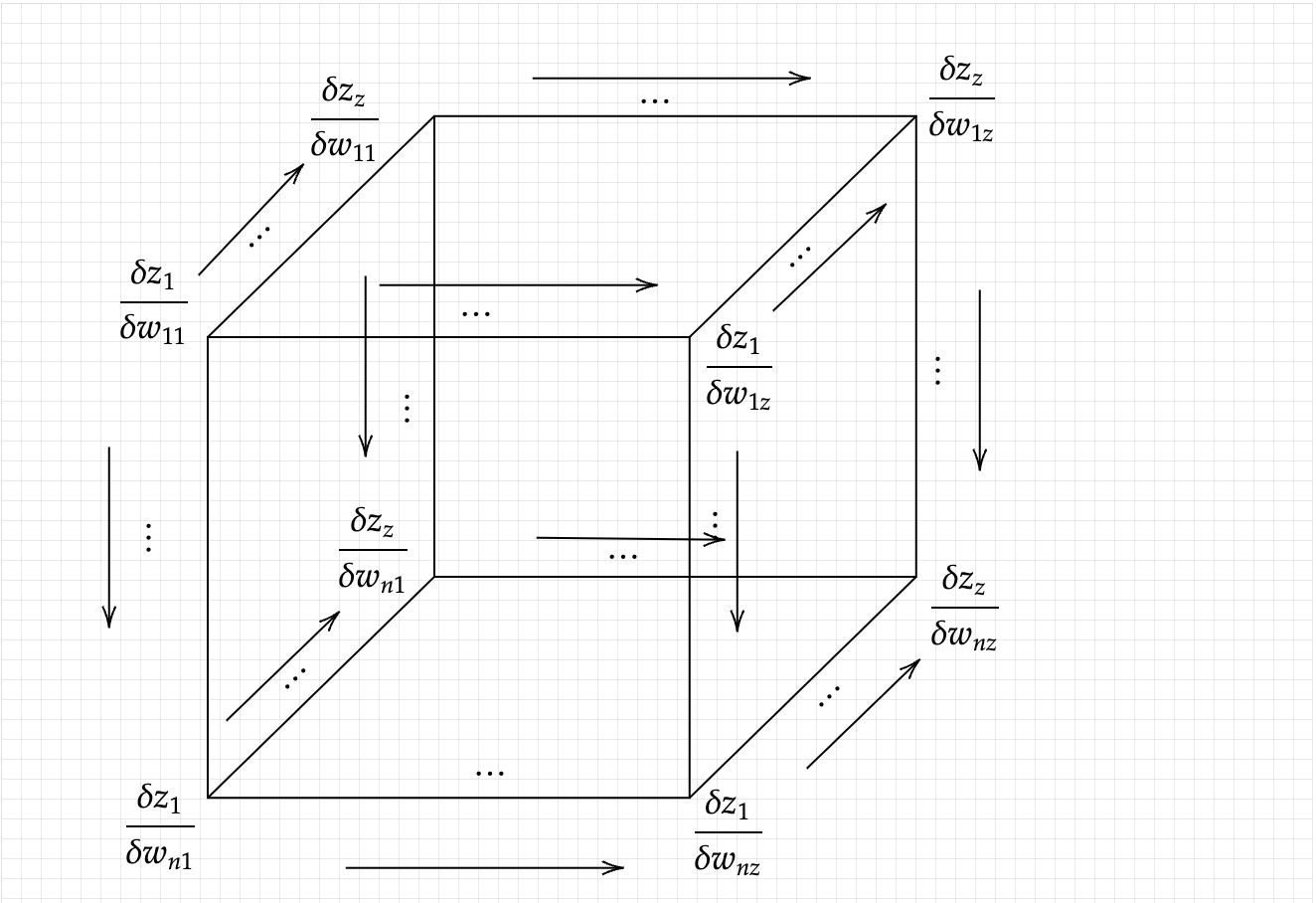
As we did before, we have to transform the Jacobian Tensor of dimensions n x z x z into a n x z matrix, with addition on the third dimension. We need to look for the overall contribution of each element of the weight matrix, namely every w_ij element of the weight matrix, hence just like before, we have,

$$\frac{\delta Z}{\delta w_{ij}}=\sum _{x=0}^z\frac{\delta z_x}{\delta w_{ij}}$$

and hence, finally we get the Jacobian Matrix of the weights, in relation with the loss function.

$$\frac{\delta Z}{\delta W}={\left[\begin{array}{ccccc}{\sum }_{x=0}^z\frac{\delta z_x}{\delta w_{11}}& {\sum }_{x=0}^z\frac{\delta z_x}{\delta w_{12}}& {\sum }_{x=0}^z\frac{\delta z_x}{\delta w_{13}}& \dots & {\sum }_{x=0}^z\frac{\delta z_x}{\delta w_{1z}}\\ {\sum }_{x=0}^z\frac{\delta z_x}{\delta w_{21}}& & & & \\ {\sum }_{x=0}^z\frac{\delta z_x}{\delta w_{31}}& & \ddots & & ⋮\\ ⋮& & & & \\ {\sum }_{x=0}^z\frac{\delta z_x}{\delta w_{n1}}& & \dots & & {\sum }_{x=0}^z\frac{\delta z_x}{\delta w_{nz}}\end{array}\right]}_{n*z}$$

And as we did before, we decrease our weight values by the Jacobian of W.

$$W^{*}=\left[\begin{array}{ccccc}{w}_{11}& w_{11}& w_{11}& \dots & w_{1z}\\ w_{21}& & & & \\ w_{31}& & \ddots & & ⋮\\ ⋮& & & & \\ w_{n1}& & \dots & & w_{nz}\end{array}\right]-\left[\begin{array}{ccccc}{\sum }_{x=0}^z\frac{\delta z_x}{\delta w_{11}}& {\sum }_{x=0}^z\frac{\delta z_x}{\delta w_{12}}& {\sum }_{x=0}^z\frac{\delta z_x}{\delta w_{13}}& \dots & {\sum }_{x=0}^z\frac{\delta z_x}{\delta w_{1z}}\\ {\sum }_{x=0}^z\frac{\delta z_x}{\delta w_{21}}& & & & \\ {\sum }_{x=0}^z\frac{\delta z_x}{\delta w_{31}}& & \ddots & & ⋮\\ ⋮& & & & \\ {\sum }_{x=0}^z\frac{\delta z_x}{\delta w_{n1}}& & \dots & & {\sum }_{x=0}^z\frac{\delta z_x}{\delta w_{nz}}\end{array}\right]$$

With this final step, we have the new weights W^* and the new baises Y^* . These new weights and biases can be used to ounce again calculate a new output, which can be again compared with the actual values, taken gradients of and repeat the process. Since the new weights and biases mathematically give us a lower loss function, in theory, if we keep doing it, we will eventaully make the loss zero (although in real-life applications, that is undesired for reasons that will not be covered here).

Continure Reading
Home