Exploring architectures- LSTMs

Introduction

As we continue to explore the current enviromment of new and better architectures in the arena of deep learning, we come across certain architectures that seem flawless: until they aren’t. One such architecture was the LSTM or the Long Short Term Memory recurrent neural network architecture, first proposed in 1997 and which remained the best in the field until a certain architecture caught our attention in 2017. LSTM was first propsed, primarily to mitigate the most prominent problems faced by recurrent neural networks at the time: the problem of exploding and vanishing gradients. To understand these, kindly go through this essay first, as it is crucial.

Exploding and Vanishing Gradients

In the previous essay I only briefly went over these problems, and now into more detail. It might not be evident through the equations from my previous essays (or any for that matter), but the reader mustn’t forget that the parameters, or any variable for that matter, are essentially matrices and could be hundreds or thousands of dimensions in size. Basically all we do during the entire process is matrix-mulplications. In this light,our gradients are matrices as well, and here we get to our problem, which is not unique to RNNs but is more prominent with them: matrix multiplication (or simply multiplication) done enough times, can either magnify a number, or diminish it completely. A simple mathematical fact has come to bite at us. During the gradient descent, in order to calculate the gradients, we go through multiple matrix multiplications … with the parameters themselves. Such are the equations, which leads to the gradients to rise exponentially, or diminish the same way. It’s not hard to see why that could be a problem: computers simply wouldn’t be able to handle numbers nearing infinity, while them nearing zero will simply mean all the information stored within is lost, leading to incorrect results. This is problematic in RNNs precisley due to their recurrent nature, gradients are used multiple times and over many layers can keep on growing or diminish rapidly. One solution was gradient clipping (introducing a threshold for gradients), but since than better techniques/architectures have emerged.

The Idea

The central idea that LSTM introduces is the usage of gates to control the flow of gradients, where there are different gates that monitor the passage of information in each cell (another word for a layer) and have different effect on the output/hidden state of the network. Like all other networks, the gates are just fully connected dense layers with mostly relu activations (we do have to use the tanh activation as well) and that is pretty much it. Apart from the simple step-by-step matrix calculations that we have to do, the basic intuition is simply to sort of restrict the flow (both forward and backward) of the weights and in turn their gradients in order to mitigate exponential growth or decay.

Gates, Nodes and Hidden States

Before we begin, we must start by devising states. From here on, each LSTM layer will be called a cell. Each cell will be fed three things: the input (X), a hidden state (H) and a memory cell internal state (C). The memory cell internal state carries information of each cell to the next, as opposed to the hidden state, which carries the input information. There are three gates inside each cell: forget, input and output, along the this cell’s internal node (like C, but of this cell). The forget gate acts on C, to determine how much of the previous cell’s information to retain and how much to flush. The input gates acts on this cell’s internal state, to determine how much should be added to the passing Memory state (C), while the output gate simply controls how this cell affects the final output. This arrangement seems abstarct and not very intuituve, as these operations seem random. But such gates help mitigate the exponential growth and decay by restricting whether each cell can affect the output or not and if yes, how much. A cell can stay non-active for a long time (forget gate is active or 1), only to suddenly become active later on, being more efficient (kind of like only being used where it’s needed). All these gates are simply dense networks, while the operations between gates is the element-wise matrix multiplication.

Initialization and Forward Propagation

Lets us start with defining our initial varialbes, namely the memory cell internal state and the hidden state. For the very first cell/layer, we can simply initialise these to be a matrix of zeros. Let X be our input or (r x d) dimensions and H and C be of (r x h) dimensions.

\begin{array}{l} 𝐗 = {[\begin{array}{ccccc} x_{11} & \dots & x_{1 d} \\ x_{21} \\ x_{31} & ⋱ & ⋮ \\ ⋮ \\ x_{r 1} & \dots & x_{r d} \end{array}]}_{r x d} 𝐇 = {[\begin{array}{ccccc} 0 & \dots & 0 \\ 0 \\ 0 & ⋱ & ⋮ \\ ⋮ \\ 0 & \dots & 0 \end{array}]}_{r x h} \\ 𝐂 = {[\begin{array}{ccccc} 0 & \dots & 0 \\ 0 \\ 0 & ⋱ & ⋮ \\ ⋮ \\ 0 & \dots & 0 \end{array}]}_{r x h} \end{array}

Next, we must initialise the weights and baises for the three gates, as well as the cell’s internal node. Remember: each gate/node is made from a dense rnn-like network, which means each has two weights (one for input one for hidden state), and a bias (six weight matrix and three bias vectors!). Not to forget the dense network for the internal node (phew, LOT of weights!).

\begin{array}{l} 𝐖_{i x} = 𝐖_{f x} = 𝐖_{o x} = 𝐖_{c x} = {[\begin{array}{ccccc} w_{11} & \dots & w_{1 h} \\ w_{21} \\ w_{31} & ⋱ & ⋮ \\ ⋮ \\ w_{d 1} & \dots & w_{d h} \end{array}]}_{d x h} \\ 𝐖_{i h} = 𝐖_{f h} = 𝐖_{o h} = 𝐖_{c h} = {[\begin{array}{ccccc} w_{11} & \dots & w_{1 h} \\ w_{21} \\ w_{31} & ⋱ & ⋮ \\ ⋮ \\ w_{h 1} & \dots & w_{h h} \end{array}]}_{h x h} \\ 𝐛_{i} = 𝐛_{f} = 𝐛_{o} = 𝐛_{c} = {[\begin{array}{c} b_{1} \\ b_{2} \\ b_{3} \\ ⋮ \\ b_{h} \end{array}]}_{1 x h}^{T} \end{array}

Given these weights, the calculation of the input gate (I), the forget gate (F), the output gate (O) and the internal node (C_i) with the relu and tanh activations is simply :

\begin{array}{l} 𝐈 = σ ({𝐗 𝐖}_{i x} + {𝐇 𝐖}_{i h} + 𝐛_{i}) \\ 𝐅 = σ ({𝐗 𝐖}_{f x} + {𝐇 𝐖}_{f h} + 𝐛_{f}) \\ 𝐎 = σ ({𝐗 𝐖}_{o x} + {𝐇 𝐖}_{o h} + 𝐛_{o}) \\ 𝐂_{i} = t a n h ({𝐗 𝐖}_{c x} + {𝐇 𝐖}_{c h} + 𝐛_{c}) \end{array}

As was mentioned before, from this cell, we get two outputs which will be passed onto the next cell: the memory cell state and the hidden state. To get to the memory cell state, first our forget gate is applied to the memory cell state of the previous cell, while the input gate acts on the internal node of this cell (remember their purpose), after we add the results, we get the new memory cell state which will be passed onto the next cell, while also being used to derive the hidden state with the help of the output gate. The sigmoid activation ensures the values of the matrix stays in the interval (0, 1) while the tanh activation ensures it stays in the interval (-1, 1).

\begin{array}{l} 𝐂_{t} = 𝐅 \times 𝐂 + {𝐈 \times 𝐂}_{i} \\ 𝐇_{t} = 𝐎 \times t a n h (𝐂_{t}) \end{array}

This procedure (‘x’ is for elementwise matrix multiplication) will give the output for a single layer. In the case of a multi-layered network, the resulting C_t and H_t will be the inputs of the next cell and the process continues to happen till we reach the output.

Backpropagation

As is the routine, we will backpropagte through these equations to find the desired gradients. In this case, we would have to find gradients for 12 parameters! Also all this for a single layer! This just goes to show why exactly neural networks require so much computational power (each calculation is a matrix multiplication as well). For more clarity, we can view the final equations as a product of just the parameters and the inputs :

Solving these by hand is tedious if we simply just start solving. Hence it is always easier to construct a computational graph, and simply work backwards through it in order to calculate the required gradients. Our final equation is not one of these, but instead our loss function. For the calculation of the loss function, we must use the cross-entropy loss. Assuming T is the true distribution (just the correct vector representation of the next letter/word/value). The cross entropy loss, is given as :

𝐋 = - (𝐓 \times l o g (𝐇) {[\begin{array}{c} 1 \\ ⋮ \\ 1 \end{array}]}_{h x 1})

Note: This may seem different than normal CE loss, but that is due to fact that I have tried to depict it purely in terms of vector notation, without using the summation symbol.

This equation is what we end up with at the end of the last LSTM layer. All we have to do is find the gradient of each parameters with respect to the above loss function. The gradients are :

\begin{array}{l} \frac{δ 𝐋}{δ 𝐖_{i x}}, \frac{δ 𝐋}{δ 𝐖_{f x}}, \frac{δ 𝐋}{δ 𝐖_{o x}}, \frac{δ 𝐋}{δ 𝐖_{o h}} \\ \frac{δ 𝐋}{δ 𝐖_{c x}}, \frac{δ 𝐋}{δ 𝐖_{i h}}, \frac{δ 𝐋}{δ 𝐖_{f h}}, \frac{δ 𝐋}{δ 𝐖_{c h}} \\ \frac{δ 𝐋}{δ 𝐛_{f}}, \frac{δ 𝐋}{δ 𝐛_{i}}, \frac{δ 𝐋}{δ 𝐛_{o}}, \frac{δ 𝐋}{δ 𝐛_{c}} \end{array}

The computational graph requires us to temporarily define some intermediate variables in order to ease the calculation of the final equation, and finding the gradients simply reduces to tracing back through the graph and calculating the required derivatives of the intermediate variables which leads us to the gradient of the weights through the chain reaction. The computational graph is given below:

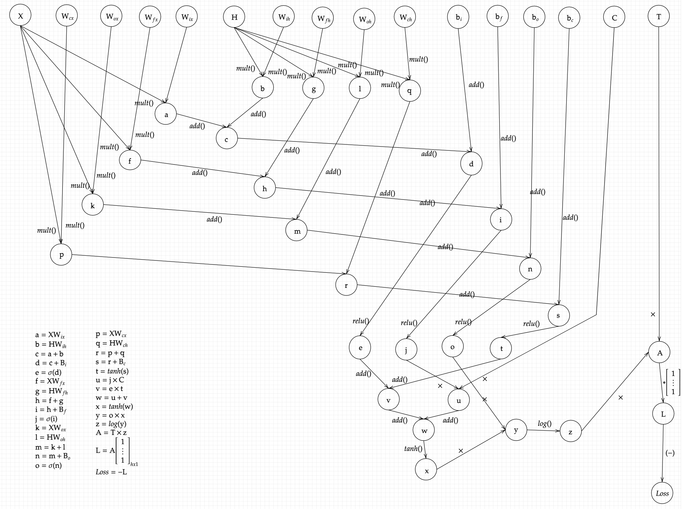
Although the graph does look quite complex, ounce we have a closer look, it is indeed trivial to solve, and makes calculating gradients not only easy but intuitive as well. The above mentioned gradients can be calculated by tracing the arrows backwards from the Loss node to each indivisual parameters, while also calculating the derivatives for the intermediate functions. This task is simple yet tedious, but here is the result:

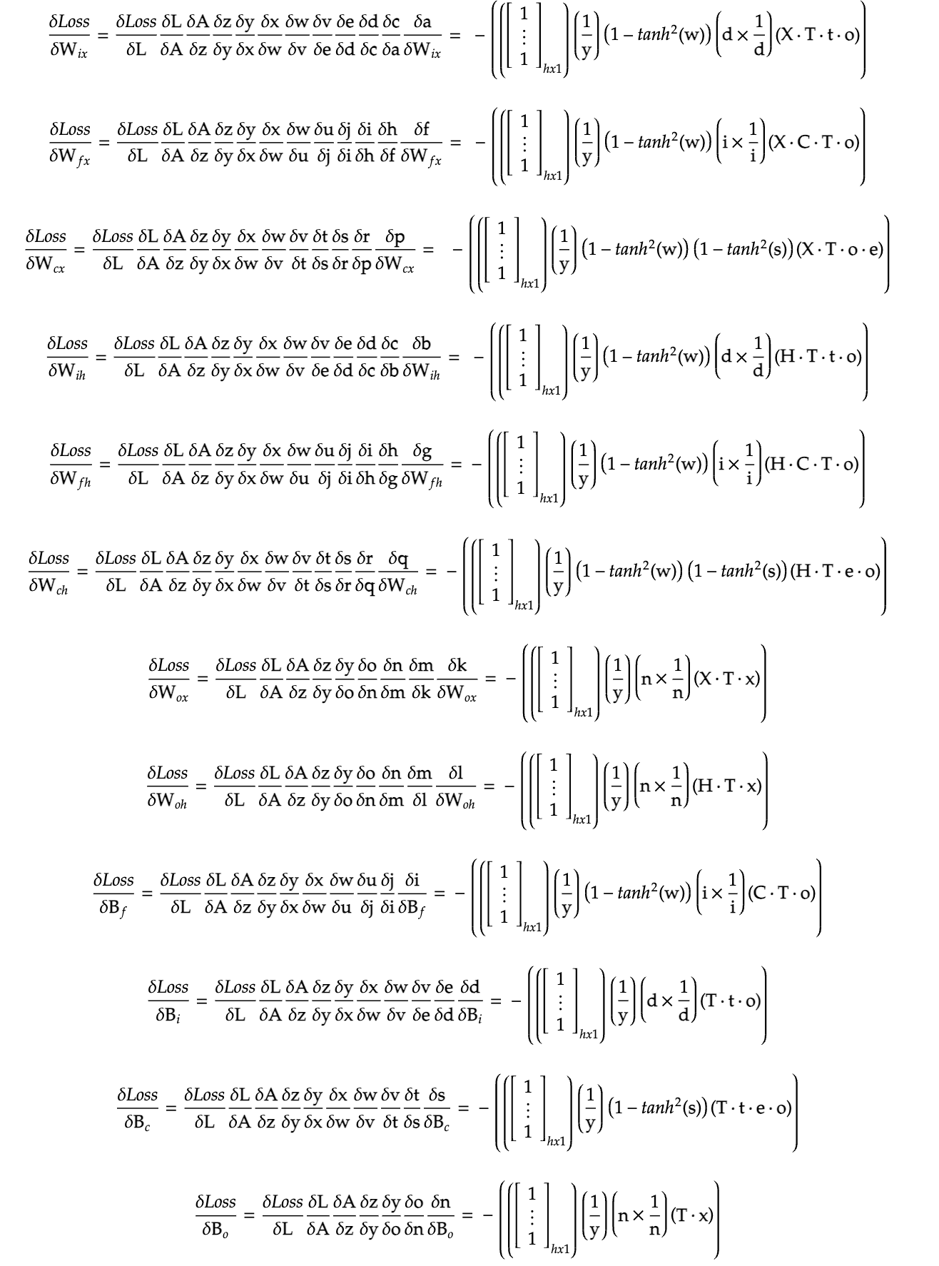
And with this, we have successfully backpropagated through a single LSTM layer. If the above equations look simple, here the first gradient purely in terms of the input, output, weights and biases.

Conclusion

The above equations can really confuse us from the real intuitions behind building these architectures, thus precaution and clarity of the concept must be mentioned. That said, this mathematical perspective could really de-mystify the seemingly magical capabalities of these networks, where we can clearly see the motivation and intention behind every operation (build through multiple essays though), and marvel at their efficiency and effectiveness in real world applications. LSTMs have been out-performed in recent times in NLP tasks, but are still rather effective in time series data. Although there are more architectures to explore, and I will continue to paint them in a simple yet intuituve mathematical perspective! Thank You.

Home