Exploring Architectures- CNN II

Building upto: Backpropagation

With our loss function defined in the previous essay, we arrive at perhaps the most important and complex part of the network (any network that is), backpropagation. We start by doing a small recap of all the operations we have done to get to our probability distribution, and put that in our loss function. As a starting point, let’s define an operation to denote a convolution, and ounce again follow the entire process (bit lenghty, but helps for revision).

\begin{array}{l} C o n v o l u t i o n a l L a y e r : 𝐈 \otimes 𝐊 : = 𝐂 \\ {[\begin{array}{ccccc} i_{1,1} & i_{1,2} & i_{1,3} & \dots & i_{1,20} \\ i_{2,1} \\ i_{3,1} & ⋱ & ⋮ \\ ⋮ \\ i_{20,1} & \dots & i_{20,20} \end{array}]}_{20 * 20} \otimes {[\begin{array}{ccc} k_{11} & k_{12} & k_{13} \\ k_{21} & k_{22} & k_{23} \\ k_{31} & k_{32} & k_{33} \end{array}]}_{3 * 3} : = {[\begin{array}{ccccc} c_{1,1} & c_{1,2} & c_{1,3} & \dots & c_{1,20} \\ c_{2,1} \\ c_{3,1} & ⋱ & ⋮ \\ ⋮ \\ c_{20,1} & \dots & c_{20,20} \end{array}]}_{20 * 20} \end{array}

\begin{array}{l} F l a t t e n i n g : 𝐂 \to 𝐂_{F} \\ {[\begin{array}{ccccc} c_{1,1} & c_{1,2} & c_{1,3} & \dots & c_{1,20} \\ c_{2,1} \\ c_{3,1} & ⋱ & ⋮ \\ ⋮ \\ c_{20,1} & \dots & c_{20,20} \end{array}]}_{20 * 20} \to {[\begin{array}{c} c_{1,1} \\ c_{1,2} \\ c_{1,3} \\ ⋮ \\ c_{20,20} \end{array}]}_{1 * 20}^{T} \end{array}

\begin{array}{l} F o r w a r d p r o p a g a t i o n I : 𝐂_{F} * 𝐖_{1} + 𝐁_{1} = 𝐎_{1} \\ {[\begin{array}{c} c_{1,1} \\ c_{1,2} \\ c_{1,3} \\ ⋮ \\ c_{20,20} \end{array}]}_{1 * 20}^{T} {[\begin{array}{ccccc} w_{1,1} & w_{12} & w_{13} & \dots & w_{1 m} \\ w_{2,1} \\ w_{3,1} & ⋱ & ⋮ \\ ⋮ \\ w_{20,1} & \dots & w_{n m} \end{array}]}_{20 * m} + {[\begin{array}{c} b_{1,1} \\ b_{1,2} \\ b_{1,3} \\ ⋮ \\ b_{20,20} \end{array}]}_{1 * m}^{T} = {[\begin{array}{c} o_{1,1} \\ o_{1,2} \\ o_{1,3} \\ ⋮ \\ o_{20,20} \end{array}]}_{1 * m}^{T} \end{array}

\begin{array}{l} A c t i v a t i o n L a y e r : R e L u (𝐎_{1}) = 𝐇 \\ \frac{1}{2} ({[\begin{array}{c} o_{1,1} \\ o_{1,2} \\ o_{1,3} \\ ⋮ \\ o_{20,20} \end{array}]}_{1 * m}^{T} + {[\begin{array}{c} | o_{1,1} | \\ | o_{1,2} | \\ | o_{1,3} | \\ ⋮ \\ | o_{20,20} | \end{array}]}_{1 * m}^{T}) = {[\begin{array}{c} h_{1,1} \\ h_{1,2} \\ h_{1,3} \\ ⋮ \\ h_{20,20} \end{array}]}_{1 * m}^{T} \end{array}

\begin{array}{l} F o r w a r d p r o p a g a t i o n I I : 𝐇 * 𝐖_{2} + 𝐁_{2} = 𝐎_{2} \\ {[\begin{array}{c} h_{1,1} \\ h_{1,2} \\ h_{1,3} \\ ⋮ \\ h_{20,20} \end{array}]}_{1 * m}^{T} {[\begin{array}{ccc} w_{11} & w_{12} & w_{13} \\ w_{21} \\ w_{31} & ⋱ & ⋮ \\ ⋮ \\ w_{m 1} & w_{m 2} & w_{m 3} \end{array}]}_{m * 3} + {[\begin{array}{c} b_{11} \\ b_{12} \\ b_{13} \end{array}]}_{1 * 3}^{T} = {[\begin{array}{c} o_{11} \\ o_{12} \\ o_{13} \end{array}]}_{1 * 3}^{T} \end{array}

\begin{array}{l} A c t i v a t i o n L a y e r : S o f t m a x (𝐎_{2}) = P^{*} (y | x; θ) \\ w h e r e, θ = {𝐖_{1}, 𝐖_{2}, 𝐁_{𝟏}, 𝐁_{2}, 𝐊} \\ σ ({[\begin{array}{c} o_{11} \\ o_{12} \\ o_{13} \end{array}]}_{1 * 3}^{T}) = {[\begin{array}{c} \frac{e^{o_{11}}}{\sum_{i = 0}^{3} e^{o_{i}}} \\ \frac{e^{o_{12}}}{\sum_{i = 0}^{3} e^{o_{i}}} \\ \frac{e^{o_{13}}}{\sum_{i = 0}^{3} e^{o_{i}}} \end{array}]}_{1 * 3}^{T} \end{array}

In the last layer, the various parameters that 𝜃 represents are simply the weights, biases and the kernel. Parameters are objects (matrices and vectors in our case) that our model used in order to arrive at the probability distribution and the ones it is allowed to tweak and adjust. The only other variables are the input and the output, which we provide and which can’t be tampered with, hence they are always constant. For the ease of backpropagation, let’s pull the variables in the loss function.

- \sum_{i} P (y | x_{i}) l o g (P^{*} (y | x_{i}; θ)))

This is the cross entropy loss. With the input layer I which is the image, we utilize the parameters W₁,W₂,B₁,B₂ and K to calculate a certain probability distribution or at least our model’s initial guess at the true distribution T. After that we simply check how wrong it was by using the cross entropy loss. Here : P^*( y | x ; 𝜃) is the probability that our model came up with using the parameters, and P(y|x) is the true probability or T.

P (y | x) = T

L o s s = - \sum T . l o g (\frac{e^{((\frac{1}{2} (I \otimes 𝐊) * 𝐖_{1} + 𝐁_{1} + | (I \otimes 𝐊) * 𝐖_{1} + 𝐁_{1} |) * 𝐖_{2} + 𝐁_{2})}}{\sum_{i} e^{{((\frac{1}{2} (i_{i} \otimes k_{i}) * w_{1 i} + b_{1 i} + | (i_{i} \otimes k_{i}) * w_{1 i} + b_{1 i} |) * w_{2 i} + b_{2 i})}_{i}}})

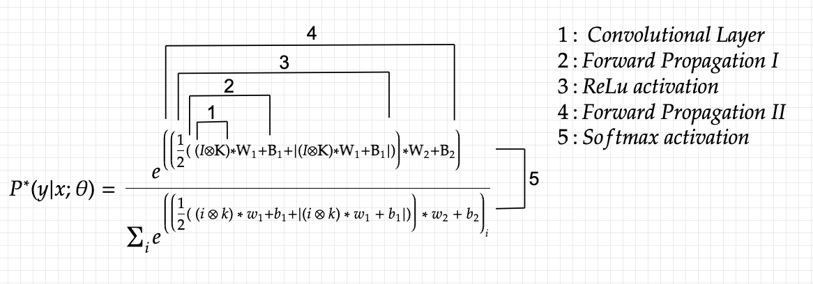
The above loss function is made up of: input I and output T, which cannot be tampered with and are constants, and parameters which the model must modify and tweak, in order to bring down the overall loss function (W₁,W₂,B₁,B₂ and K). The reason the above equation looks so complicated is due to the fact that I put each and every variable in terms of either the input or one of the parameters. It need not be so complicated, but since mathematical theory requires it (and it’s fun as well), I tried my best. Perhaps the most difficult part is yet to come: we must find the derivative of the loss function with respect to each of the parameters, in order to perform gradient descent optimization.

Backpropagation

As discussed in previous essays, the above derived loss function must be minimized. But how ? In order to answer that question, we must remember how it was formed in the first place: through the use of certain parameters (mathematical objects of our/model’s desire) and real world data that we obtained (I and T for input and the actual true values of the output). We adjust the parameters after every iteration in such a way that it minimizes the loss function. By how much should be change the parameters? By the loss’s derivative with respect to the parameters. This is one of the most important optimization algorithms in deep learning, known as gradient descent optimization. (For further details, read my previous essayhere).

For us to solve the various gradients with respect to our inputs by hand is already a very tedious task: as we have an already very complex loss function with multiple inputs. But nevertheless, I have broken down the equation into various parts and constructed a computational graph for the same, where we can more easily see what’s happening under the hood and also easily calculate derivatives of more simpler functions and than to pile them up. First we start by assigning sub-variables and creating what we call a computational graph (I would highly recommend readingthis essay before going on, as it will make things crystal clear).

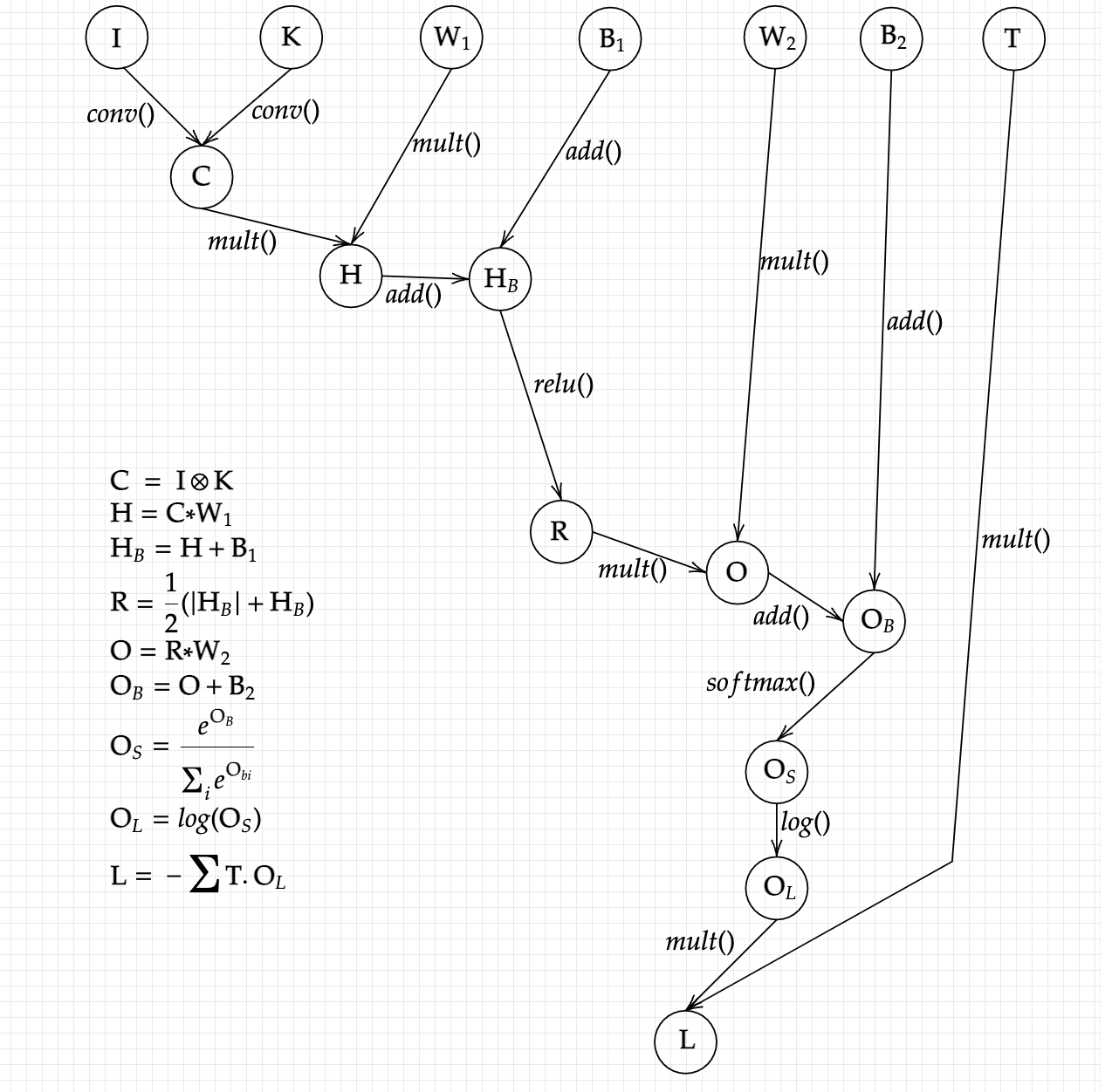
Thus we have formed our graph, with each sub-variable repesenting an operation performed on our original parameters or Input in order to reach our output. This view is much simpler, and makes it easier to get to the next step, where we want to calculate each variable’s gradient with respect to the variable that were used in creating it. Before that, let’s view notationaly what we want: the derivative of the Loss function with respect to W₁, B₁, W₂, B₂, K.

\frac{δ L o s s}{δ 𝐁_{2}}, \frac{δ L o s s}{δ 𝐖_{2}}, \frac{δ L o s s}{δ 𝐁_{1}}, \frac{δ L o s s}{δ 𝐖_{1}}, \frac{δ L o s s}{δ 𝐊}

In order to get to these, we just need to traverse the graph backwards and get to the final output, hence backpropagation. Since the values are too complex, I have first calculated the indivisual gradients of sub-variables as follows:

\begin{array}{l} \frac{δ 𝐋}{δ 𝐎_{L}} = - i 𝐓, \frac{δ 𝐎_{L}}{δ 𝐎_{S}} = \frac{\sum_{i} e^{{((\frac{1}{2} ((i \otimes k) * w_{1} + b_{1} + | (i \otimes k) * w_{1} + b_{1} |)) * w_{2} + b_{2})}_{i}}}{e^{((\frac{1}{2} ((I \otimes 𝐊) * 𝐖_{1} + 𝐁_{1} + | (I \otimes 𝐊) * 𝐖_{1} + 𝐁_{1} |)) * 𝐖_{2} + 𝐁_{2})}} \\ \frac{δ 𝐎_{S}}{δ 𝐎_{B}} = [\begin{array}{c} 𝐎_{1} - 𝐎_{1} . 𝐎_{1}^{T} - \sum_{\begin{array}{l} j \\ j \neq 1 \end{array}} 𝐎_{1} . 𝐎_{j} \\ 𝐎_{2} - 𝐎_{2} . 𝐎_{2}^{T} - \sum_{\begin{array}{l} j \\ j \neq 2 \end{array}} 𝐎_{2} . 𝐎_{j} \\ 𝐎_{i} - 𝐎_{i} . 𝐎_{i}^{T} - \sum_{\begin{array}{l} j \\ j \neq i \end{array}} 𝐎_{i} . 𝐎_{j} \end{array}], w h e r e 𝐎_{i} = \frac{e^{{((\frac{1}{2} ((I \otimes 𝐊) * 𝐖_{1} + 𝐁_{1} + | (I \otimes 𝐊) * 𝐖_{1} + 𝐁_{1} |)) * 𝐖_{2} + 𝐁_{2})}_{i}}}{\sum_{i} e^{{((\frac{1}{2} ((i \otimes k) * w_{1} + b_{1} + | (i \otimes k) * w_{1} + b_{1} |)) * w_{2} + b_{2})}_{i}}} \\ \frac{δ 𝐎}{δ 𝐖_{2}} = \frac{1}{2} ((I \otimes 𝐊) * 𝐖_{1} + 𝐁_{1} + | (I \otimes 𝐊) * 𝐖_{1} + 𝐁_{1} |) \\ \frac{δ 𝐑}{δ 𝐇_{B}} = \frac{1}{2} ((I \otimes 𝐊) * 𝐖_{1} + 𝐁_{1} + | (I \otimes 𝐊) * 𝐖_{1} + 𝐁_{1} |) \\ \frac{δ 𝐂}{δ 𝐊} = {[\begin{array}{ccc} c_{11} & \dots & c_{1 n} \\ ⋮ & ⋱ & ⋮ \\ c_{n 1} & \dots & c_{n n} \end{array}]}_{n * n}, \frac{δ 𝐇}{δ 𝐖_{1}} = I \otimes 𝐊 \\ \frac{δ 𝐇}{δ 𝐂} = 𝐖_{1}, \frac{δ 𝐎}{δ 𝐑} = 𝐖_{2} \\ \frac{δ 𝐇_{B}}{δ 𝐇} = 1, \frac{δ 𝐇_{B}}{δ 𝐁_{1}} = 1, \frac{δ 𝐎_{B}}{δ 𝐎} = 1, \frac{δ 𝐎_{B}}{δ 𝐁_{2}} = 1 \end{array}

And finally, through the chain rule, we get to our final parameter gradients:

\begin{array}{l} \frac{δ 𝐋}{δ 𝐁_{2}} = \frac{δ 𝐋}{δ 𝐎_{L}} \frac{δ 𝐎_{L}}{δ 𝐎_{S}} \frac{δ 𝐎_{S}}{δ 𝐎_{B}} \frac{δ 𝐎_{B}}{δ 𝐁_{2}} \\ \frac{δ 𝐋}{δ 𝐖_{2}} = \frac{δ 𝐋}{δ 𝐎_{L}} \frac{δ 𝐎_{L}}{δ 𝐎_{S}} \frac{δ 𝐎_{S}}{δ 𝐎_{B}} \frac{δ 𝐎_{B}}{δ 𝐎} \frac{δ 𝐎}{δ 𝐖_{2}} \\ \frac{δ 𝐋}{δ 𝐁_{1}} = \frac{δ 𝐋}{δ 𝐎_{L}} \frac{δ 𝐎_{L}}{δ 𝐎_{S}} \frac{δ 𝐎_{S}}{δ 𝐎_{B}} \frac{δ 𝐎_{B}}{δ 𝐎} \frac{δ 𝐎}{δ 𝐑} \frac{δ 𝐑}{δ 𝐇_{B}} \frac{δ 𝐇_{B}}{δ 𝐁_{1}} \\ \frac{δ 𝐋}{δ 𝐖_{1}} = \frac{δ 𝐋}{δ 𝐎_{L}} \frac{δ 𝐎_{L}}{δ 𝐎_{S}} \frac{δ 𝐎_{S}}{δ 𝐎_{B}} \frac{δ 𝐎_{B}}{δ 𝐎} \frac{δ 𝐎}{δ 𝐑} \frac{δ 𝐑}{δ 𝐇_{B}} \frac{δ 𝐇_{B}}{δ 𝐇} \frac{δ 𝐇}{δ 𝐖_{1}} \\ \frac{δ 𝐋}{δ 𝐊} = \frac{δ 𝐋}{δ 𝐎_{L}} \frac{δ 𝐎_{L}}{δ 𝐎_{S}} \frac{δ 𝐎_{S}}{δ 𝐎_{B}} \frac{δ 𝐎_{B}}{δ 𝐎} \frac{δ 𝐎}{δ 𝐑} \frac{δ 𝐑}{δ 𝐇_{B}} \frac{δ 𝐇_{B}}{δ 𝐇} \frac{δ 𝐇}{δ 𝐂} \frac{δ 𝐂}{δ 𝐊} \end{array}

By substituting the above equations with their actual values, we see that the gradients are indeed quite complex, despite us dealing with a fairly rudimentry network. All that remains is that we change the parameters by their gradients and keep continuing the process until we reach a desired loss level.

Ok. That was a lot of calculations and maths to deal with ! This entire process discussed above and in the previous essay constitutes the convolutional nueral network, which gives computers vision. More sophiticated models are far more complex and larger in their parameter size and numbers (as many might know, chatGPT has 175 billion paramters, compared to the measly five we used here). But no model strays too far away from the basic architecture, and hence we always benefit from knowing these architectres inside out. Believe it or not, the entire process above can be acheived in just a few lines of code using certain deep learning framworks (PyTorch or Tensorflow). Anyways, thank you for reading this far!

Home