Automatic Differentiation II

In the last essay, we saw how we can calculate the gradients of scalar functions, by implementating backpropagation through a graph data structure. The implementation process was preceded by the theory behind both the graph data structure and the chain rule. The final algorithm was very useful in calculating scalar values, but we must not forget multi-dimensional inputs. At times (most of the times actually), we need gradients on vector valued functions, not scalar. Therefore, in this continuation essay, we shall explore Vector calulus and how it fits in Automatic Differentiation.

Vector Calculus

There isn’t as much difference in this topic, compared to normal calculus. Topics that are generally taught under this concept such as Divergence, Curl, Line Integrals .. etc. won’t be covered here (anyone interested can exploreKhan academy, for their excellent courses), as they are not relevant in ML/DL. We shall only go over the general cases, and put them in our algorithm. A vector is simply a list of numbers put together,

$$x=\left[\begin{array}{ccccc}{x}_1& x_2& x_3& \dots & x_n\end{array}\right],xϵ{ℝ}^n$$

Where R denotes the set of all real numbers. What we are interested in, is what is the derivative of a vector with respect to another vector. As I covered this in another essay as well (Neural Networks through Linear Algebra), it results in what we call a Jacobian. Let v and x be two vectors,

$$\begin{array}{l}𝐯=\left[\begin{array}{ccccc}{v}_1& v_2& v_3& \dots & v_n\end{array}\right],𝐯ϵ{ℝ}^n\\ \\ \\ \\ x=\left[\begin{array}{ccccc}{x}_1& x_2& x_3& \dots & x_m\end{array}\right],xϵ{ℝ}^m\end{array}$$

If we need to find out the derivative of v with respect to x, we get a Jacobian Matrix.

$$\frac{\delta 𝐯}{\delta 𝐱}={\left[\begin{array}{ccccc}\frac{\delta v_1}{\delta x_1}& \frac{\delta v_2}{\delta x_1}& \frac{\delta v_3}{\delta x_1}& \dots & \frac{\delta v_n}{\delta x_1}\\ \\ \frac{\delta v_1}{\delta x_2}& & & & \\ \\ \frac{\delta v_1}{\delta x_3}& & \ddots & & ⋮\\ \\ ⋮& & & & \\ \\ \frac{\delta v_1}{\delta x_m}& & \dots & & \frac{\delta v_n}{\delta x_m}\end{array}\right]}_{n*m}$$

Generally when we deal with multi-dimensional data, we need to pay special attention to the dimensions. In the above example, we see how the matrix combines the dimensions of the two vectors, to give us an *n * m* dimensional matrix. The reason is simple: we simply calculated the derivative of each element in v with respect to each element in x, and put them all in the matrix. When it comes to the derivative of a matrix with respect to a vector, the same process applies, and we get a three-dimensional Jacobian cube structure. But a more easier process would be to simply reshape the matrix into a vector. Let M be a matrix, of dimensions *r * y*.

$$𝐌={\left[\begin{array}{ccccc}{m}_{11}& m_{21}& m_{31}& \dots & m_{x1}\\ \\ m_{12}& & & & \\ \\ m_{13}& & \ddots & & ⋮\\ \\ ⋮& & & & \\ \\ m_{1y}& & \dots & & m_{xy}\end{array}\right]}_{r*y}$$

Reshaping the matrix into a vector would give us a vector of ry dimensions. This can be done because there exists an isomorphism (they are similiar, or have similiar/same properties) between R^{*r * y*} and R^ry. The matrix M after reshaping looks like this,

$$𝐌=\left[\begin{array}{cccccccccccc}{m}_{11}& m_{12}& m_{13}& \dots & m_{1y}& m_{21}& \dots & m_{2y}& \dots & m_{x1}& \dots & m_{ry}\end{array}\right]𝐌ϵ{ℝ}^{ry}$$

After reshaping, calculating the derivative with respect to any other vector is simply to follow the previous steps, to get a Jacobian matrix.

$$𝐌=\left[\begin{array}{ccccc}{m}_1& m_2& m_3& \dots & m_{ry}\end{array}\right],𝐌ϵ{ℝ}^{ry}$$

$$\frac{\delta 𝐌}{\delta 𝐱}={\left[\begin{array}{ccccc}\frac{\delta m_1}{\delta x_1}& \frac{\delta m_2}{\delta x_1}& \frac{\delta m_3}{\delta x_1}& \dots & \frac{\delta m_{ry}}{\delta x_1}\\ \\ \\ \\ \frac{\delta m_1}{\delta x_2}& & & & \\ \\ \\ \\ \frac{\delta m_1}{\delta x_3}& & \ddots & & ⋮\\ \\ \\ \\ ⋮& & & & \\ \\ \\ \\ \frac{\delta m_1}{\delta x_m}& & \dots & & \frac{\delta m_{ry}}{\delta x_m}\end{array}\right]}_{ry*m}$$

Doing so, we basically get the same Jacobian cube as before, as you can check with the dimensions (*r * y * m* = *ry * m*), because all we did was reshape the matrix for easier calculations and understanding. With this, we can move forward to see how to backpropagate with vector-valued functions.

Backpropagation with Vectors

As we did before, it would benefit us if we applied this theory with a numerical example in mind. Let us define two vectors,

$$\begin{array}{l}𝐱=\left[\begin{array}{ccccc}1.0& 3.0& 6.0& 2.0& 0.0\end{array}\right],xϵ{ℝ}^5\\ \\ 𝐲=\left[\begin{array}{ccccc}2.0& 7.0& 5.0& 1.0& 1.0\end{array}\right],yϵ{ℝ}^5\end{array}$$

And going further, we can define an equation using them as our primary variable,

$$\begin{array}{l}𝐳={𝐱}^{\mathrm{𝟐}}+{𝐲}^{\mathrm{𝟐}}\\ \\ \\ \\ 𝐳={\left(\left[\begin{array}{ccccc}1.0& 3.0& 6.0& 2.0& 0.0\end{array}\right]\right)}^2+{\left(\left[\begin{array}{ccccc}2.0& 7.0& 5.0& 1.0& 1.0\end{array}\right]\right)}^2\\ \\ \\ \\ 𝐳=\left[\begin{array}{ccccc}5.0& 58.0& 61.0& 5.0& 1.0\end{array}\right],zϵ{ℝ}^5\end{array}$$

Thus we have the value of z vector, with the dimensions being (1 x 5). Going further, before we begin with calculating the gradients, let’s visualize it in a graph data structure, where we need two more sub-variables: u = x² and v = y²

$$\begin{array}{l}𝐮=\left[\begin{array}{ccccc}1.0& 9.0& 36.0& 4.0& 0.0\end{array}\right]\\ \\ 𝐯=\left[\begin{array}{ccccc}4.0& 49.0& 25.0& 1.0& 1.0\end{array}\right]\end{array}$$

Upto here, we are in similiar territory as scalar valued functions. But as we shall see, while backpropagating from here, we observe a change in dimensions which needs to be dealt with. Going back as usual leads us to the following equations:

$$\begin{array}{l}\frac{\delta 𝐳}{\delta 𝐮}=1,\frac{\delta 𝐳}{\delta 𝐯}=1\\ \\ \\ \\ \frac{\delta 𝐮}{\delta 𝐱}=2𝐱=\left[\begin{array}{ccccc}2.0& 6.0& 12.0& 4.0& 0.0\end{array}\right],\\ \\ \\ \\ \frac{\delta 𝐯}{\delta 𝐲}=2𝐲=\left[\begin{array}{ccccc}4.0& 14.0& 10.0& 2.0& 2.0\end{array}\right]\\ \\ \\ \\ \frac{\delta 𝐳}{\delta 𝐱}=\frac{\delta 𝐳}{\delta 𝐮}\frac{\delta 𝐮}{\delta 𝐱}=2𝐱\\ \\ \\ \\ \frac{\delta 𝐳}{\delta 𝐲}=\frac{\delta 𝐳}{\delta 𝐯}\frac{\delta 𝐯}{\delta 𝐲}=2𝐲\end{array}$$

As was in the previous essay, the graph looks like this:

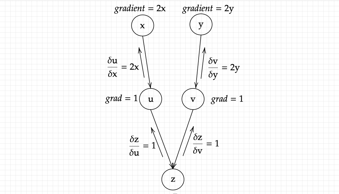
One thing that we must remember is that the expressions of partial derivatives represent matrices and not simple vectors. This can prove somewhat troublesome while implementing practically, as the gradients as passed backwards, they are needed for further computations, which can become complicated quickly as the dimensions increase rapidly, and sort of accumulate. For instance,

$$\frac{\delta 𝐳}{\delta 𝐮}={\left[\begin{array}{ccccc}\frac{\delta z_1}{\delta u_1}& \frac{\delta z_2}{\delta u_1}& \frac{\delta z_3}{\delta u_1}& \frac{\delta z_4}{\delta u_1}& \frac{\delta z_5}{\delta u_1}\\ \\ \\ \\ \frac{\delta z_1}{\delta u_2}& & & & \\ \\ \\ \\ \frac{\delta z_1}{\delta u_3}& & \ddots & & ⋮\\ \\ \\ \\ \frac{\delta z_1}{\delta u_4}& & & & \\ \\ \\ \\ \frac{\delta z_1}{\delta u_5}& & \dots & & \frac{\delta z_5}{\delta u_5}\end{array}\right]}_{5*5}$$

Is already a matrix R^{*5 * 5*}, and will be used to calculate the gradients as we go further up the graph, and be multiplied by other matrices. Apart from that, if we had started x or y to be matrices, it would have resulted in the same difficulty. Due to this reasons, we utilize a gradient tensor at the beginning of the algorithm. It is nothing but a vector passed onwards from the starting point, following the same process as before.

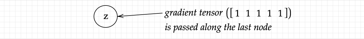
Passing along this vector won’t change our answers at all, for example, our Jacobian was J_x (or J_y), and with passing along this vector, we simply end up with [1, 1, 1, 1, 1]^T. J_x , which will give us the original vector (the gradient of x or y), as doing the above mentioned operations reduces the matrix to a vector, which is what we desired in the first place (the dimension are (*1 * 5*) x (*5 * 5*) = *1 * 5*), giving us a vector. The main reason for passing in a vector in the last node was to reduce our output from a matrix to a vector, or whatever the dimension was of our input. Note that the gradient tensor has to match the dimensions of the function value (z).

Another added advantage is that we get control over the sensitivity of the output with respect to the input. If instead we passed in a gradient tensor [1, 1, 2, 1, 1], we will get the same output, except the third element will be twice of the original answer, as was intended. Overall, passing in a gradient tensor proves quite useful when calculating gradients of vector-valued functions. With this, we are done with the theory for Automatic Differentiation !

Home