Automatic Differentiation

Computing derivatives can be useful and necessary in many fields, and yet difficult to actually implement. Standing apart from other methods for computing derivaitves, Automatic Differentiation is the most accurate we can get. There are multiple reasons for using this technique, some of them are: it plays right into a computer’s strength of performing simple operations on a variable or two, it provides accurate results, at least compared to other methods and due to it’s structure is very convenient for calculating gradients (derivatives or simply slope) of multiple inputs. A major use case is in artificial intelligence, namely Deep Learning, where familiarity with automatic differentiation is a must, and major frameworks are made just for the ease of calculating derivatives (plus other data science stuff). According to naming conventions, it is called autograd (automatic gradients) and thus will be referred to as such henceforth. AutoGrad relies on two things: the mathematical theory of chain rule and the computer science theory of graphs, and how we can implement them both in order to create what we want. We shall go over the theories below.

Mathematical Theory: The Chain Rule

While we might implement through code how to differentiate different equations, we should also gain some insight into why certain techniques work, and the mathematical reason behind them. It’ll benefit us with the understanding of how and why autograd works, and under what principles it does so. The chain rule, is simply a way to get the derivaitve of complex functions, where there might be functions inside functions, for example,

$$f(x)=sin(log(x))$$

As sin() and log() are both functions, the chain rule guides us on how to solve these type of complex functions. It is a very simple procedure, ignore the “inner” function (log() in this case) and solve the outer function, then find the derivative of the inner function, and simple multiply.

$$\frac{d}{dx}sin(log(x))=cos(log(x))*\frac{1}{x}$$

This allows us to seperate each function into it’s simplest part (x²,log()), solve them and just multiply the answers back together. This process is very similiar to recursion in computer science, and hence can be exploited to easily calculate the derivatives of any function. Lets look at the same example, but with a bit of substitution. Let u = log(x) and v=*sin(u)*, so v is our original function.

$$\begin{array}{l}\frac{\delta }{\delta x}v=\frac{\delta }{\delta x}sin(𝐮)=cos(𝐮)*\frac{\delta }{\delta x}𝐮[thechainrule]\\ \\ \\ \\ \frac{\delta }{\delta x}𝐮=\frac{\delta }{\delta x}log(x)=\frac{1}{x}\\ \\ \\ \\ \frac{\delta }{\delta x}sin(log(x))=cos(𝐮)*\frac{1}{x}=cos(log(x))*\frac{1}{x}[substituting𝐮back]\end{array}$$

The complex function was broken down into two simple ones,*cos(u)* and log(x), solved, and their answers put together to get the final product. The chain rule. How does this help us simplify and implement autograd ? We look into every complex function until we come across a very basic operation, like addition or multiplication or log() or sin(), and solve them easily (since we already know the answers through pre-determined formulae) and put all the answers together, like above, and get to the final product.

Computer Science Theory: Graphs

In order to effectively use various theoritical ideas, algorithms and techniques in computers and practically using them, they must be implemented with well-defined structures. This is where the second part of autograd comes in: the usage of a graph data structure. A graph is very common in it’s usage, and has thus also found it’s way into autograd. It consists of two sub-parts: a node and an edge. In theory, a node can be any defined structure. It can be a function or a number or any other object we define, while an edge is simply a connection between two different nodes. In our case, a node will simply be a number or an array (in case of multiple inputs), and the edge will be the operation that will connect it to another node, i.e, array or number. For instance, in 3 + 5 = 8, all of the numbers are nodes, while the addition operation is the edge. Diagrammatically, it’ll be like this :

This is a very simple example of a graph. The nodes can be anything, while the edges can go in any direction. The meaning of the edges can change according to how we define the graph, such as,

Here, the edge is defined as the subtraction operation. We can now get some vague idea about how this could relate to the technique of autograd. There is another CS concept: recursion algorithm, which will be looked into during implementation itself. Now, how do graphs fit into autograd ? As we discussed before, autograd technique looks into every complex function’s sub-part till it reaches the very basic operation done on the primary variable. A better way to understand will be to look at the above solved complex function through the lens of graphs, where as before, we take v=*sin(u)* and u=log(x).

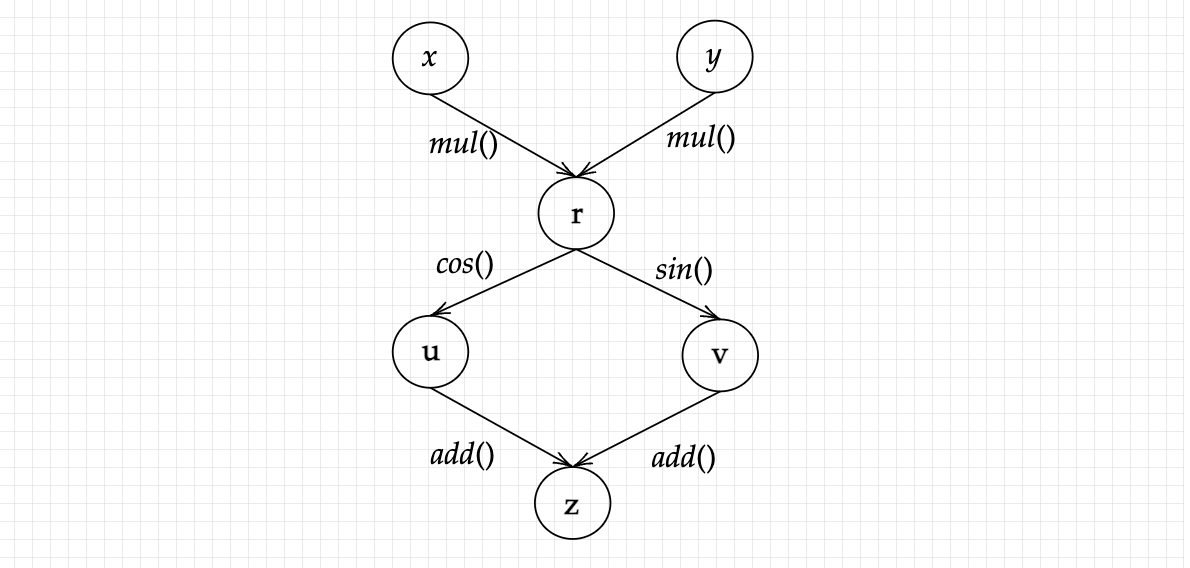
And thus, we arrive at our complex function. Here we can see that our variables are the nodes and the operations are the edges connecting these nodes. Before we get done with the this section, let’s take a look at what happens when we use multiple inputs. Suppose we’ve another equation but with multiple inputs: f(x,y) = sin(xy) + cos(xy) . How will this be represented ? Do not forget that we have multiplication as one of the primary operations ! More complex functions have more sub-variables assigned to them. Let’s use variables for ease in representing:

$$\begin{array}{l}𝐳=sin(xy)+cos(xy)\\ \\ \\ 𝐯=sin(xy)\\ \\ \\ 𝐮=cos(xy)\\ \\ \\ 𝐫=xy\end{array}$$

These are our variables. Now let’s represent them as a graph data structure:

This is how a complex function with multi-variable input is represented as a graph. The variables and sub-variables are all nodes, while all the operations are the edges that connect these nodes to each other. We indirectly program these graphs, and utilize the connections to calculate the derivatives or gradients of each indivisual input.

Combining the two: Backpropagation

Now we move on to the final part: calculating the gradient, or the derivative of our function. An advantage we have is we just have to trace back our steps along the graph in order to calculate our gradient, with respect to each of the given inputs! Before starting, we must clarify our end goal: we need the gradients of x and y, with respect to z. We can calculate this easily by hand, as shown in the Mathematical Theory section, but for computers, a graph data structure can not only make things more plausable, but also give them enough efficiency and computational power to calculate extremely complex derivatives, something that is in-feasible for humans to do by hand. Before starting, it’ll help to give certain values to x and y, as we can than simply trace this numerical value backwards. Therefore, let x = 2 and y = 3. Than by extension:

$$\begin{array}{l}𝐫=2*3=6\\ \\ \\ 𝐮=cos(6)\approx 0.96\\ \\ \\ 𝐯=sin(6)\approx -0.27\\ \\ \\ 𝐳=0.96-0.27\approx 0.69\end{array}$$
We have,

$$\begin{array}{l}𝐳=𝐮+𝐯\\ \\ \\ 𝐮=cos(𝐫),𝐯=sin(𝐫)\\ \\ \\ 𝐫=xy\end{array}$$

Therefore we start our process from z, where,

$$\begin{array}{l}\frac{\delta 𝐳}{\delta x}=\frac{\delta 𝐳}{\delta 𝐮}\frac{\delta 𝐮}{\delta 𝐫}\frac{\delta 𝐫}{\delta x}+\frac{\delta 𝐳}{\delta 𝐯}\frac{\delta 𝐯}{\delta 𝐫}\frac{\delta 𝐫}{\delta x}=\frac{\delta 𝐫}{\delta x}(\frac{\delta 𝐳}{\delta 𝐮}\frac{\delta 𝐮}{\delta 𝐫}+\frac{\delta 𝐳}{\delta 𝐯}\frac{\delta 𝐯}{\delta 𝐫})\\ \\ \\ \\ \\ \frac{\delta 𝐳}{\delta x}=y(cos(xy)-sin(xy))[substituting𝐫back]\\ \\ \\ \\ \\ \frac{\delta 𝐳}{\delta y}=\frac{\delta 𝐳}{\delta 𝐮}\frac{\delta 𝐮}{\delta 𝐫}\frac{\delta 𝐫}{\delta y}+\frac{\delta 𝐳}{\delta 𝐯}\frac{\delta 𝐯}{\delta 𝐫}\frac{\delta 𝐫}{\delta y}=\frac{\delta 𝐫}{\delta y}(\frac{\delta 𝐳}{\delta 𝐮}\frac{\delta 𝐮}{\delta 𝐫}+\frac{\delta 𝐳}{\delta 𝐯}\frac{\delta 𝐯}{\delta 𝐫})\\ \\ \\ \\ \\ \frac{\delta 𝐳}{\delta y}=x(cos(xy)-sin(xy))[substituting𝐫back]\end{array}$$

Going further, we calculate the indivisual values:

$$\begin{array}{l}\frac{\delta 𝐳}{\delta 𝐮}=\frac{\delta (𝐮+𝐯)}{\delta 𝐮}=1\frac{\delta 𝐳}{\delta 𝐯}=\frac{\delta (𝐮+𝐯)}{\delta 𝐯}=1\\ \\ \frac{\delta 𝐮}{\delta 𝐫}=\frac{\delta cos(𝐫)}{\delta 𝐫}=-sin(𝐫)=0.27\frac{\delta 𝐯}{\delta 𝐫}=\frac{\delta sin(𝐫)}{\delta 𝐫}=cos(𝐫)=0.96\\ \\ \frac{\delta 𝐫}{\delta x}=\frac{\delta xy}{\delta x}=y=3\frac{\delta 𝐫}{\delta y}=\frac{\delta xy}{\delta y}=x=2\end{array}$$

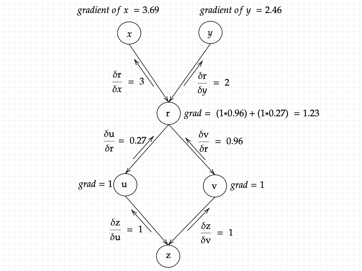
The above given answer is an important expression: it is our gradient, constructed piece by piece using the numerical values we have provided. Writing such equations side by side overcomplicates things, so let’s visualize these through graphs. To represent each gradient accumulated at the node, I’ll use grad.

The above graph should make things clear about how the gradients are calculated, how they accumulate in the variable r, before going on to give us each seperate gradients of x and y. Precisely what makes this algorithm so powerful is it’s ability to calculate multiple derivatives, or derivaties of multiple inputs all at ounce. We simply have to write an equation, and start the backpropagation process! The algorithm will accurately calculate each partial derivative value, putting computer’s biggest strength of automation to good use. But we are far from over: this algorithm, as it is, is useful for scalar values only: we need to take into account multi-dimensional inputs as well, hence enter Vector Calculus. We shall look into it in the next essay !

Continure Reading
Home